Importance Sampling
DISCLAIMER: This is a blog post from my graduate school years. The blog is no longer maintained and the material might include typos and errors.
Suppose we want to calculate the integral
\[\text{E}_f[g(Y)] =\int_{\mathcal Y} g(y) f(y) dy < \infty,\]where $ Y $ is a random variable with pdf $ f $, $ \mathcal Y =\{y \in \mathbb R \, \vert \, f(y) >0\}$, and $ g: \mathbb R \rightarrow \mathbb R $ is a real-valued function. In words, it means that we are interested in the expectation of a function of the random variable $Y$.
Even if we are not able to calculate the expectation analytically, we might approximate the expectation by the Monte Carlo estimate
\[\hat\mu_{\text{MC}} = \frac{1}{S}\sum_{s=1}^S g(y^{(s)})\]in situations where we are able to obtain $ S $ simulation draws from $ f $, which we denote by $y^{(s)}, s = 1,2,…,S$. By the (Strong) Law of Large Numbers, $ \hat\mu_{\text{MC}}$ converges (almost surely) to $ \text{E}_f[g(Y)] $ as the expectation is finite and the draws are independent. So, by sampling many times we can get an arbitrarily precise estimate of $\text{E}_f[g(Y)]$.
However, in many other situations, even sampling from $f$ is not possible or inefficient. Importance sampling can be used to overcome this limitation if there is another distribution $ q $ that satisfies the following conditions:
- $q$ has support on $ \mathcal Q \subseteq \mathbb R $;
- we are able to obtain random draws from $q$; and
- for all $y \in \mathcal Q,$ $g(y)f(y) > 0$ implies that $q(y) > 0. $ That is, in regions the integrand, $g \cdot f$, is positive, the “proposal density”, $q$, has to be positive as well.
Notice that it follows from condition (3) that $ g(y)f(y) = 0 $ if $ y\in \mathcal Y \Delta \mathcal Q $, where $ A\Delta B $ is the symmetric difference between sets $ A $ and $ B $. It follows that
\[\begin{aligned} \text{E}_f[g(Y)] &= \int_{\mathcal Y} g(y) f(y) dy \\ &= \int_{\mathcal Y \cap \mathcal Q} g(y)f(y) dy + \int_{\mathcal Y \Delta \mathcal Q} g(y)f(y) dy \\ & = \int_{\mathcal Q } g(y)f(y) dy = \int_{\mathcal Q} g(y)\left[\frac{f(y)}{q(y)}\right]q(y)dy = \text{E}_q\left[\frac{g(Y)f(Y)}{q(Y)}\right] \\ &= \text{E}_q\left[g(Y)w(Y)\right],\end{aligned}\]where $ w(Y) = f(Y)/q(Y) $. Therefore, we can approximate the expectation by
\[\hat\mu_{\text{IS}} = \frac{1}{S} \sum_{s=1}^S w^{(s)} g(y^{(s)})\]with $ S $ independent samples drawn from $ q $ (not $ f $) and where $ w^{(s)} = f(y^{(s)})/q(y^{(s)}) $. Intuitively speaking, the ratios $ w^{(s)} $, called importance ratios, compensates for the fact that we are sampling from $ q $ instead of $ p $ when estimating the desired expectation. Furthermore, $ \hat\mu_{\text{IS}} $ converges a.s. to $ \text{E}_q\left[\frac{g(Y)f(Y)}{g(Y)}\right] $ and thus to $ \text{E}_p[g(Y)] $.
Unknown Proportionality Constant
Importance sampling can also be used when $ f $ is known only up to a constant. These situations often arise in Bayesian analysis where $ f = p_{\text{post}}^\ast $ is the unnormalized posterior of $ \theta $, the parameter of interest. That is, $ p_{\text{post}}^\ast(\theta \, \vert \, x) = L(x \, \vert \, \theta) p_{\text{prior}}(\theta) $ where $ L(x\, \vert \, \theta) $ is the likelihood of the data $ x $ and $ p_{\text{prior}}(\theta) $ the prior distribution.
Let $ f^\ast $ be the unnormalized density of $ f $ and denote by $ k $ the proportionality constat such that $ f = k\cdot f^\ast $. Further, define the unnormalized importance ratios, $ w^\ast (y): \mathcal Y \rightarrow \mathbb R $ as $ w^\ast(y) = f(y)^\ast / q(y) = k \cdot w(y) $ to sample from $ f $. Then
\[\frac{\int_{\mathcal Y} g(y)w^\ast(y)q(y) dy}{\int_{\mathcal Y} w^\ast(y)q(y)dy} = \frac{k \int_{\mathcal Y} g(y)w(y) q(y) dy}{k\int_{\mathcal Y} w(y)q(y)dy} = \int_{\mathcal Y} g(y)w(y) q(y) dy = \text{E}_f[g(Y)].\]The proportionality constants in the numerator and denominator cancel each other out, and $ \int_{\mathcal Y} w\cdot q = \int_{\mathcal Y} (f /q ) q = \int_{\mathcal Y} f = 1 $ as $ f $ is a probability distribution. What is left, therefore, is the desired expectation. It follows that we can use the estimator
\[\hat\mu_{\text{IS}} = \frac{\frac{1}{S} \sum_{s=1}^S w^{*(s)} g(y^{(s)})}{\frac{1}{S}\sum_{s=1}^S w^{*(s)}}\]where $ w^{*(s)} = f^\ast(y^{(s)})/q(y^{(s)}) $. Notice that this ratio-estimator is not unbiased, since, in general, $ \text{E}[X/Y] \ne \text{E}[X]/\text{E}[Y] $. The estimator is, however, consistent as numerator converges to $ \text{E}[g(Y)] $ and the denominator to 1. Also, note that the estimator works even if both $ f $ and $ q $ are known only up to a constant. If $ k $ and $ c $ are the proportionality constants for $ f $ and $ q $, respectively, both the numerator and the denominator in the expression above will have $ k/c $ as a factor, which, again, cancel each other out.
A Panacea?
Of course, importance sampling is not a panacea. In fact, it can go seriously off. To see why this is so, let $ \theta = \int_{\mathcal Y}g(y)f(y) dy $ and assume that the draws from $ q $ are independent. Then the variance of the estimator $ \hat\mu_{\text{IS}} $ is
\[\begin{aligned} \text{Var}_q[\hat\mu_{\text{IS}}] &= \text{Var}_q\left[\frac{1}{S} \sum_{s=1}^S W(Y^{(s)}) g(Y^{(s)})\right] \\ &= \frac{1}{S} \text{Var}_q\left[W(Y) g(Y)\right]\\ &=\frac{1}{S}\Big\{\text{E}_q\left[\left(W(Y) g(Y)\right)^2\right] - \theta^2\Big\}\\ &= \frac{1}{S}\left\{ \int_{\mathcal Q} \left[ \frac{g(y)f(y)}{q(y)} \right]^2 q(y) dy - \theta^2 \right\} \end{aligned}\]where the first step follows from the fact that $ y^{(s)} $ are iid samples from $ q $. This expression shows that although $\hat{\mu}_{\text{IS}} \rightarrow \text{E}_f[g(Y)]$, the variance of $ \hat{\mu}_{\text{IS}} $ will be finite only if
\[\text{E}_q\left[\left(\frac{g(Y)f(Y)}{q(Y)}\right)^2\right] = \int_{\mathcal Q}\left[g(y)^2f(y)\right]\left[\frac{f(y)}{q(y)}\right] dy < \infty.\]Thus, the ratio $ w = f/q $ is crucial to obtain reliable estimates with finite samples. For instance, if the tails of $ q $ are lighter than that of $ f $, leading to unbounded ratios $ w = f/q $ in the tails of $ Y $, the variance of $ \hat\mu_{\text{IS}} $ will blow up. In other words, just any distribution $ q $ from which we can sample is not enough, and we have to choose $ q $ carefully.
Efficiency Gains
In fact, it turns out that by choosing a “good” proposal distribution $ q $, it is possible to obtain an estimator with lower variance than $ \hat\mu_{\text{MC}} $. A straightforward example is the following. Suppose we are interested in $ \mu = E_f[g(Y)] $ where $ Y \sim \text{Normal}(0,1) $ and $ g(Y) = \mathbb I(Y>1.96) $. If we use $ S $ samples from a standard normal and calculate $ \mu_{\text{MC}} $, the variance of the estimator is
\[\text{Var}_f[\hat\mu_{\text{MC}}] = \text{Var}\left[\frac{1}{S} \sum_{s=1}^S \mathbb I(Y^{(s)}> 1.96)\right] \approx \frac{39}{1600S}\]as $ \theta = \text{E}_f[\mathbb I(Y^{(s)} > 1.96)] \approx \frac{1}{40} $ and $ \text{Var}_f[\mathbb I(Y^{(s)} > 1.96)] = \theta(1-\theta) $. This way of simulating the tail-probability is actually quite inefficient as many of the generated samples will be smaller than 1.96 and have, therefore, only limited information regarding the expectation we are trying to calculate.
So, consider another approach (which will turn out to be a bad choice). We might try to exploit the fact that the normal distribution is symmetric and write
\[\text{E}_f[\mathbb I(Y>1.96)] = \int_{-\infty}^\infty \mathbb I(y>1.96) f(y) dy = \frac{1}{2} - \int_{0}^{\infty}\mathbb I(y<1.96)f(y)dy.\]To evaluate the integral, we use $ q \sim \text{Uniform}(0,1.96) $ which satisfies the condition that $ g(y)f(y) = 1\cdot f(y) =0 $ whenever $ q(y) =0 $ on $ (0,1.96) $. Thus,
\[\text{E}_f[\mathbb I(Y> 1.96)] = \frac{1}{2} - \int_{0}^{\infty} \mathbb I(y < 1.96)\left[\frac{f(y)}{q(y)}\right]q(y) dy = \frac{1}{2} - 1.96 \int_{0}^{1.96}f(y)q(y) dy,\]and we can use importance sampling with:
\[\hat\mu_{\text{IS}} = \frac{1}{2} - \frac{1.96}{S}\sum_{s=1}^S f(y^{(s)}),\]where $ {y^{(s)}}_{s=1}^S $ are draws from the $ \text{Uniform(0,1.96)} $ distribution. The variance of this estimator can be derived analytically as well.
\[\begin{aligned} \text{Var}_q[\hat\mu_{\text{IS}}] & = \frac{1.96^2}{S}\text{Var}_q[f(Y)] = \frac{1.96}{S}\int_{0}^{1.96}\frac{1}{\sqrt{2\pi}}e^{-y^2/2}dx \\ &= \frac{1.96}{S}\left(\Phi(1.96) - \frac{1}{2}\right) \\ &\approx \frac{.2256}{S}, \end{aligned}\]where $ \Phi(\cdot) $ is the standard normal cdf. Unfortunately, the result suggests that the “uniform trick” will result in an estimator with larger variance than $ \text{Var}_f[\hat\mu_{\text{MC}}]$, so this is not a good approach…
Let us give it another try. Notice that the variance of the importance sampling estimator is a function of $ z(y) = [g(y)f(y)]^2/q(y) \ge 0 $. This means that to reduce the variance of $ \hat\mu_{\text{IS}} $ we need to choose a distribution $ q $ that is large for those regions of $ \mathcal Y $ in which $ g(y)f(y) $ is large. As we have $g(y) = \mathbb I(Y > 1.96)$, it follows that $z(y) = 0$ for $y < 1.96$, implying that we don’t need to care about that region. For $y>1.96$, we note that the normal density $f(y)$ is a strictly decreasing function in $y$. Hence by choosing $q$ such that it has its mode near $1.96$ and is decreasing for $y> 1.96$, although at a slower rate than the normal density, we might be able to find an estimator with small variance.
Here, we consider two distributions: the $ \text{Exponential}(\lambda) $ distribution with pdf
\[q(y; \lambda) = \lambda e^{-\lambda y}, \qquad \lambda > 0, y > 0,\]and the $ \text{Shifted-Exponential}(\lambda, \gamma) $ distribution which can be defined stochastically as follows: if $ X\sim \text{Exponential}(\lambda) $, then $ Z = \gamma + Y $ has a $ \text{Shifted-Exponential}(\lambda,\gamma) $ distribution. The pdf of a Shifted-Exponential distribution with parameters $ \lambda $ and $ \gamma $ is given as
\[q(y; \lambda, \gamma) = \lambda e^{-\lambda (y - \gamma)}, \qquad \lambda, \gamma > 0, x > \gamma.\]Let us first plot the considered proposal distributions and the normal distribution on $ \mathbb R_+ $, where we use the parameters $ \lambda = 1 $ for the Exponential distribution and $(\lambda = 1, \gamma = 1.96)$ for the Shifted Exponential distribution. Notice that the exponential distribution will have its mode at $ 0 $ and a mean of $ 1 $. The shifted-exponential, on the other hand, will have its mode at $ 1.96 $ and a mean of $ 2.96 $ (recall that the exponential distribution is memoryless).
First, we load some packages.
library('ggplot2')
library('dplyr')
library('data.table')
library('dtplyr')
library('viridis')
The proposal distributions look as follows:
# set theme for plots

theme_set(theme_bw())

# generate data

data.table(x = seq(0, 10, .05))[
 , c('Normal',
     'Exponential',
     'Shifted-Exponential'
     ) :=
      list(
        dnorm(x),
        dexp(x),
        ifelse(x > 1.96, dexp(x - 1.96), NA)
      )
] %>%

  # melt into long-format

  melt(
    id.vars = 'x',
    variable.name = 'Distributions',
    value.name = 'Density'
  ) %>%

  # drop missings (shift-exp)

  filter(!is.na(Density)) %>%

  # plot distributions

  ggplot(
    aes(x = x, y = Density, col = Distributions)
  ) +
  geom_vline(xintercept = 1.96, linetype = 2) +
  geom_line() +
  scale_color_viridis(end= .8, discrete = T) +
  labs(x='',
       caption = 'Note: Vertical line shows Y = 1.96') +
  ggtitle('Normal, Exponential, and Shifted-Exponential Distribution')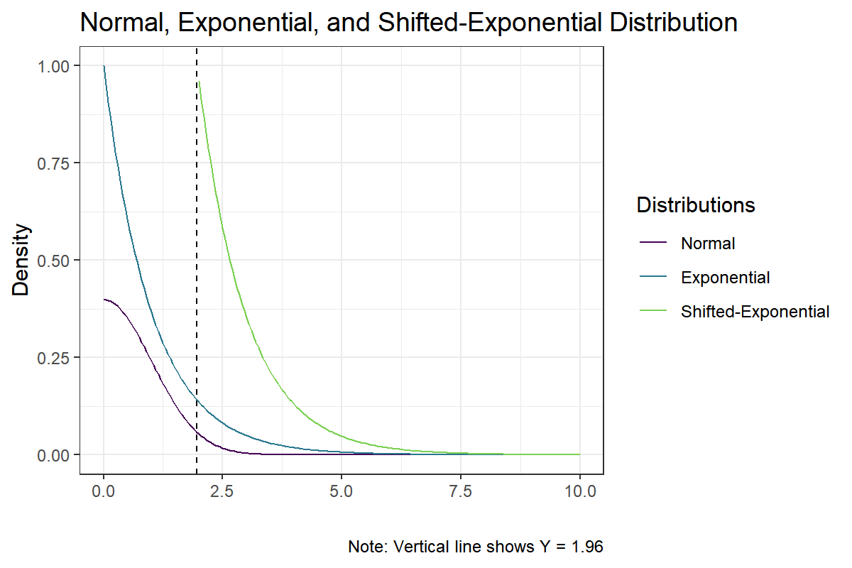
Notice that both the exponential and the shifted-exponential distribution dominate the normal distribution on $ (1.96,\infty) $. By construction, the importance sampling estimator using either of the proposal distributions will be unbiased and consistent. Yet, the shifted-exponential distribution, compared to the standard exponential distribution, has a much higher density in regions where $ f $ tends to be relatively large. This should bring efficiency gains to the estimator.
Simulations: Successful Case
To compare the performance importance sampling using different proposal distributions, we can run a simple simulation. For all that follows, we draw n.draws = 1,000 samples from the normal and the proposal distributions and calculate the Monte Carlo estimate. We repeat this process n.sim = 5,000 times and calculate the variance of each estimator across the repeated runs.
# set seed

set.seed(1987)

# number of draws from f

n.draws <- 5000

# number of simulations

n.sim <- 1000

# tail probability Y > 1.96

theta <- pnorm(1.96, lower.tail = F)

# function to generate proposals

gen.proposal <- function(f, n.draws, n.sim , ...) {

  # input  f       = distribution to draw from

  #        n.draws = number of draws per simulation

  #        n.sim   = number of simulation runs

  #        ...     = optional arguments for f

  # output         = a n.draws X n.sim matrix of

  #                 random draws, so that each

  #                 column is a independent run


  matrix(
    f(n.sim * n.draws, ...), nrow=n.draws, ncol=n.sim
  )
}


# Direct Simulation ------------------------------


# function g(Y)

g <- function (y) y > 1.96
# simulate n.draws * n.sim normal variates

x <- gen.proposal(rnorm, n.draws, n.sim)
# get mean for each simulation

mu.mc <- colMeans(g(x))

# Uniform(0, 1.96) Distribution ------------------


# simulate n.draws*n.sim uniform(0, 1.96) variates

q <- gen.proposal(runif, n.draws, n.sim, 0, 1.96)
# importance sampling estimator

mu.uniform <- .5 - 1.96*colMeans(dnorm(q))

# Exponenetial(1) Distribution -------------------


# generate draws from exp(1)

q <- gen.proposal(rexp, n.draws, n.sim)
# importance ratios

w <- dnorm(q) / dexp(q)
# estimates

mu.exp <- colMeans(g(q) * w)

# Shifted Exponential(1, 1.96) Distribution ------


q <- gen.proposal(rexp, n.draws, n.sim) + 1.96
w <- dnorm(q) / dexp(q - 1.96)
mu.shiftexp <- colMeans(g(q)* w)
Next, let’s plot the results
df <- data.table(
  x = c(mu.mc, mu.uniform, mu.exp, mu.shiftexp)
)

df[, Distributions := rep(
    c('Simple Monte Carlo',
      'Uniform',
      'Exponential',
      'Shifted-Exponential'
      ),
    each = n.sim
  )
]

# plot results

ggplot(df, aes(x = x, fill = Distributions)) +
  geom_vline(xintercept = theta,
             size = .5,
             linetype = 2) +
  geom_density(alpha = .5, size = .6, col= 'white') +
  scale_fill_viridis(end = .8, discrete = T) +
  labs(x = '',
       y = 'Density',
       caption = bquote(
         'Note: Vertical line shows true value of E['~g(Y)~']')
  ) +
  ggtitle(
    bquote(.(n.draws)~'Monte Carlo estimates of E['~g(Y)~']')
  )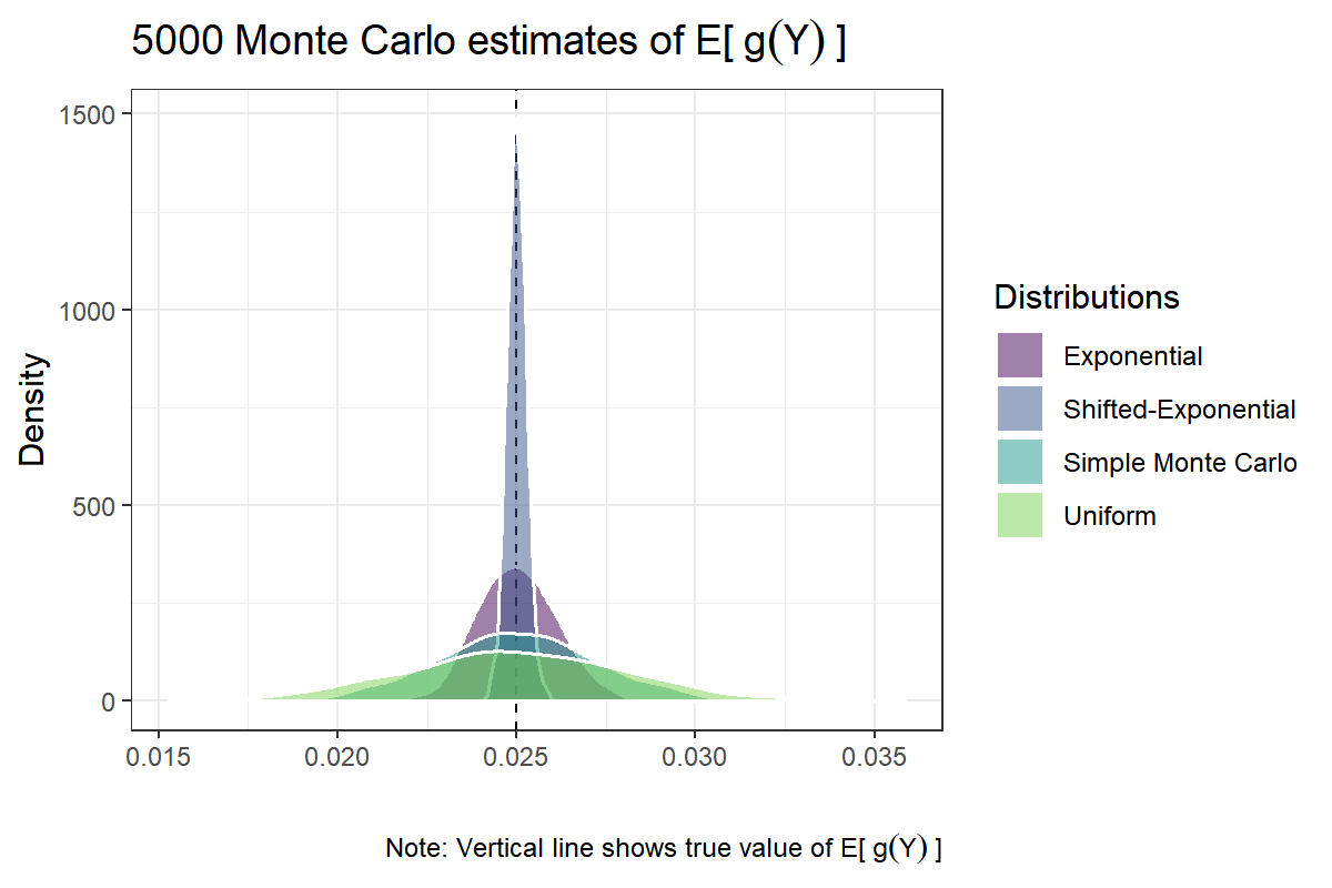
The results show how a good choice of the proposal distribution $ q $ can greatly reduce the variance of the Monte Carlo estimator. All estimators are concentrated near the true value of $ \text{E}_f[g(Y)] \approx .025 $. Also, consistent with our analytical results, the vanilla Monte Carlo approach performs better, in terms of variance, then importance sampling using the uniform distribution. Yet, importance sampling using the shifted-exponential distribution, by far, outperforms the other estimators.
Simulations: Failed Case
Next, let us consider an example in which importance sampling does a really poor job. As noted above, using importance sampling can lead to trouble if the proposal density $ q $ is small in regions where $ f $ is large. So let us consider a case in which $ f\sim \text{Normal}(0,1) $ and $ q\sim \text{Normal}(0, \sigma) $, with $ \sigma $ set to $ .25 $, $ .5 $ and $ .75 $, and lastly $ q\sim \text{Cauchy}(0,1) $. Further let $ g: x\mapsto x^4 $, i.e., the fourth moment the standard normal distribution, for which we know in advance that the true value is $ \text{E}_f[X^4] = 3 $. This time, let’s first rely on simulation to see what happens if $ f $ has heavier tails than $ q $ (as we have the code now ..). Thereafter, we might try to get some analytical insights.
# function g(Y)

g <- function(y) y^4

pars <- list(
  c('norm', 0, .25),
  c('norm', 0, .50),
  c('norm', 0, .75),
  c('cauchy', 0, 1)
)

# generate simulations

sim.res <- lapply(pars, function(w) {
  d <- switch(w[[1]],
              'norm' = c(rnorm, dnorm),
              'cauchy' = c(rcauchy, dcauchy)
              )
  opts <- as.numeric(unlist(w[2:3]))
  q <- gen.proposal(d[[1]], n.draws, n.sim, opts[1], opts[2])
  w <- dnorm(q) / d[[2]](q, opts[1], opts[2])
  # save both the estimates and w

  list(mc = colMeans(w * g(q)), w = w)
})

# get MC estimates

df <- lapply(sim.res, `[[`, 1) %>%
  # stack into a long vector

  do.call(c,.) %>%
  # generate data.table

  data.table(x = .)

# add labels

df[
    , Proposals := rep(
        c('Normal(0,.25)',
          'Normal(0,.5)',
          'Normal(0,.75)',
          'Cauchy(0,1)'
          ),
        each = n.sim
      )
  ]

# plot results

ggplot(df, aes(x = x, fill = Proposals)) +
  geom_vline(xintercept = 3,
             size = .5,
             linetype = 2) +
  geom_density(alpha = .5, size = .6, col= 'white') +
  scale_fill_viridis(end = .8, discrete = T) +
  labs(x = '',
       caption = bquote(
          'Note: Vertical line shows true value of E['~Y^4~']'
         )
  ) +
  ggtitle(
    bquote(.(n.draws)~'Monte Carlo estimates of E['~Y^4~']')
  ) +
  xlim(0,5)
## Warning: Removed 87 rows containing non-finite values (stat_density).
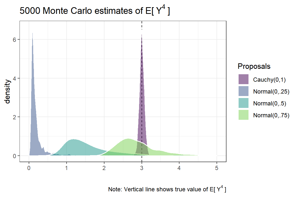
Notice that the problem with relatively thin-tailed proposal distributions is not only that of variance but that they also appear to be badly off. Summary statistics of the Monte Carlo estimates using different proposal distributions are shown below:
df[, as.list(summary(x)), by = Proposals]## Proposals Min. 1st Qu. Median Mean 3rd Qu.
## 1: Normal(0,.25) 0.03498268 0.08812097 0.1276078 0.4667546 0.2127324
## 2: Normal(0,.5) 0.62692832 1.14786265 1.4558909 2.5741800 2.0037231
## 3: Normal(0,.75) 1.92276460 2.52270543 2.7972547 3.0949051 3.1722653
## 4: Cauchy(0,1) 2.74354689 2.95936040 3.0005385 3.0021985 3.0451249
## Max.
## 1: 60.932357
## 2: 448.135139
## 3: 47.224083
## 4: 3.234684
The estimator using the $ \text{Normal}(0,.75) $ as proposal seem to hit the mark, on average, but the distribution is still skewed with a median at 2.77. When we choose even narrower proposals, $ \text{Normal}(0,.5) $ or $ \text{Normal}(0,.25) $, the results are even worse. Only for the $ \text{Cauchy}(0,1) $ proposal is the importance sampling estimator behaving reasonably. What’s going wrong? Asymptotically, $ \hat\mu_{\text{IS}} $ should converge to $ \text{E}_p[g(Y)] $. This result holds true. The problem is that we will never have infinite samples; and in this example, even n.draws=5,000 seems not enough for the estimator to converge, except for the Cauchy distribution.
Let us look a little bit deeper into the failed case of $ q \sim \text{Normal}(0, .75) $. Let us increase the number of draws per simulation from $ 5,000 $ to $ 500,000 $. Unfortunately, due to my 5-year old laptop with limited RAM, we are forced reduce the number of simulations to $ 500 $.
# number of draws

draw.nums <- c(1000, 5000, 10000, 50000, 250000)
# reduce simulation runs ;(

n.sim <- 500

df.75 <- lapply(
  draw.nums,
  function(w) {
    q <- gen.proposal(rnorm, w, 500, 0, .75)
    w <- dnorm(q)/dnorm(q, 0, .75)
    mu <- colMeans(w * g(q))
  }
) %>%
  do.call(cbind, .) %>%
  data.table %>%
  setnames(paste0('draws = ', draw.nums)) %>%
  .[, sim.no := .N] %>%
  melt(id.vars = 'sim.no')

ggplot(df.75, aes(x=value, fill = variable)) +
    geom_vline(xintercept = 3,
             size = .5,
             linetype = 2) +
    geom_density(alpha = .5, size = .6, col= 'white') +
    scale_fill_viridis(name = 'No. of Draws',
                       end = .8, discrete = T) +
    labs(x = '',
         caption = bquote(
            'Note: Vertical line shows true value of E['~Y^4~']'
           )
    ) +
    ggtitle(
      bquote('Monte Carlo estimates of E['~Y^4~']'),
      'Using proposal distribution Normal(0, .75)'
    ) +
    xlim(0,10)
## Warning: Removed 50 rows containing non-finite values (stat_density).
## Warning: Removed 7 rows containing non-finite values (stat_density).
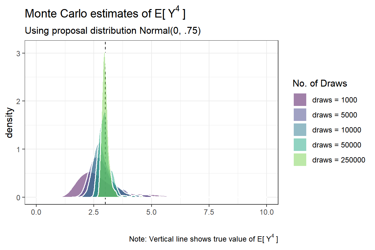
Even for $ 250,000 $ draws the distribution is slightly skewed. However, it is apparent from the plot that the familiar Central Limit Theorem is kicking in: namely the distribution of the estimator is slowly, but certainly, becoming bell-shaped with more Monte Carlo samples.
df.75[, as.list(summary(value)), by = variable]## variable Min. 1st Qu. Median Mean 3rd Qu. Max.
## 1: draws = 1000 1.282201 2.136475 2.584598 3.029645 3.330171 41.820763
## 2: draws = 5000 1.887612 2.484827 2.783248 3.033615 3.168243 25.392484
## 3: draws = 10000 2.076658 2.605695 2.809937 2.934698 3.111567 18.786551
## 4: draws = 50000 2.515928 2.794577 2.943229 2.982500 3.078682 5.742313
## 5: draws = 250000 2.711354 2.893530 2.975565 3.004073 3.071075 5.359459
Notice also that even with n.draws = 1,000 the average over repeated simulation runs hits the mark, which is expected from a consistent estimator. The variance of the sampling distribution decreases with more draws as well.
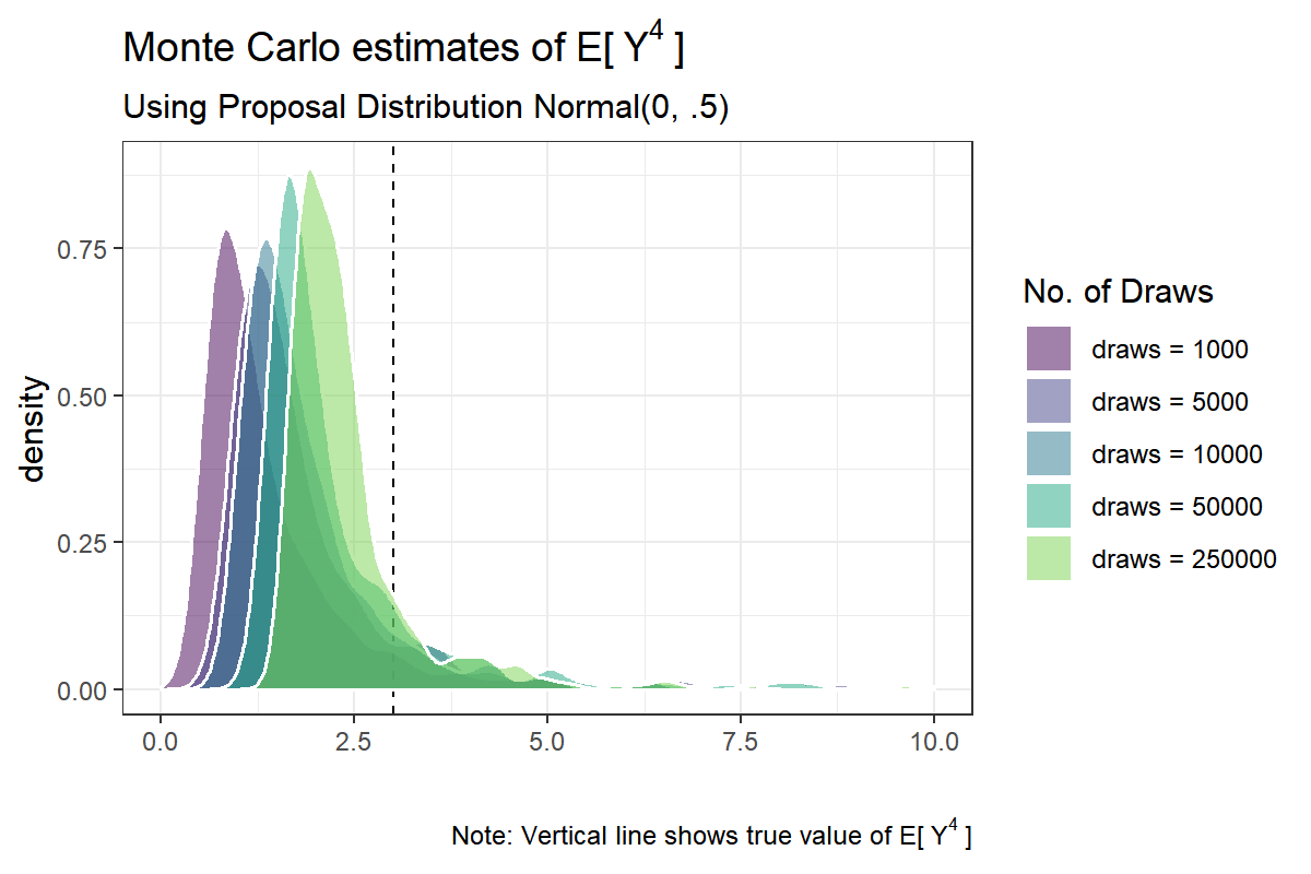
Let us compare this result with the $ \text{Normal}(0,.5) $ proposal:
draw.nums <- c(1000, 5000, 10000, 50000, 250000)

df.50 <- lapply(
  draw.nums,
  function(w) {
    q <- gen.proposal(rnorm, w, 500, 0, .5)
    w <- dnorm(q)/dnorm(q, 0, .5)
    mu <- colMeans(w * g(q))
  }
) %>%
  do.call(cbind, .) %>%
  data.table %>%
  setnames(paste0('draws = ', draw.nums)) %>%
  .[, sim.no := .N] %>%
  melt(id.vars = 'sim.no')

ggplot(df.50, aes(x=value, fill = variable)) +
    geom_vline(xintercept = 3,
             size = .5,
             linetype = 2) +
    geom_density(alpha = .5, size = .6, col= 'white') +
    scale_fill_viridis(name = 'No. of Draws',
                       end = .8, discrete = T) +
    labs(x = '',
         caption = bquote(
            'Note: Vertical line shows true value of E['~Y^4~']'
           )
    ) +
    ggtitle(
      bquote('Monte Carlo estimates of E['~Y^4~']'),
      'Using Proposal Distribution Normal(0, .5)'
    ) +
    xlim(0,10)

df.50[, as.list(summary(value)), by = variable]
## Warning: Removed 50 rows containing non-finite values (stat_density).
## Warning: Removed 7 rows containing non-finite values (stat_density).
##          variable      Min.   1st Qu.   Median     Mean  3rd Qu.      Max.
## 1:   draws = 1000 0.3771995 0.7982266 1.127576 2.074887 1.826450  40.06564
## 2:   draws = 5000 0.6812313 1.1815376 1.547561 3.940681 2.237010 730.20317
## 3:  draws = 10000 0.7967879 1.2919215 1.623777 2.757038 2.181835 191.05582
## 4:  draws = 50000 1.1518128 1.6016889 1.870101 2.448241 2.510181  49.34133
## 5: draws = 250000 1.4105277 1.8969605 2.186513 3.569468 2.559615 467.75247
This doesn’t look good. The distributions are skewed and remain skewed even for n.draw = 250,000. As $ \hat{\mu}_{\text{IS}} $ is consistent, the average over simulation runs should become closer to the true mean as n.draws is increased. But the summary statistics indicate that even n.draws = 250,000 might not be enough. Further, although the distribution seems to move slowly towards its target, it is hard to discern whether the spread of the distribution is narrowing down, remaining stable, or becoming larger; the average across simulations is also hovering around the true value but varies quite a lot even with many MC samples.
Some Analytical Insights
Why do the results differ so much? In the case of $ \text{Normal}(0,.75) $ and the $ \text{Normal}(0, .5) $ proposals, we can analyze the results analytically. We know that $ \text{E}_f[g(Y)] $ is finite as $ f $ is a standard normal distribution for which all moments are finite. So, let us focus on $ w(Y) = f(Y)/q(Y) $.
Let us denote by $ \phi(y; \sigma) $ the normal pdf with mean $ 0 $ and standard deviation $ \sigma $. By construction, $ \text{E}_q[w(Y)] = \int_{\mathcal Q} w(y) \phi(y; \sigma_q) dy = \int_{\mathcal Y} \phi(y; \sigma_f) dy = 1 $. Thus $ \text{Var}_q[\hat\mu_{\text{IS}}] $ will depend on the second moment:
\[\begin{aligned} \text{E}_q[w(Y)^2] &= \int [w(y)]^2 \phi(y;\sigma_q) dy \\ &= \int \frac{\phi(y;\sigma_f)^2}{\phi(y;\sigma_q)} dy \\ &= \int w(y) \phi(y; \sigma_f) dy \\ &= \int \frac{\sigma_q}{\sigma_f}\exp\left[-\frac{y^2}{2}\left(\frac{ \sigma_q^2 - \sigma_f^2 }{\sigma_f^2\sigma_q^2}\right)\right] \phi(y;\sigma_f) dy \\ &= \frac{\sigma_q}{\sqrt{2\pi}\sigma_f^2}\int \exp\left[-\frac{y^2}{2}\left( \frac{2}{\sigma_f^2}- \frac{1}{\sigma_q^2}\right)\right] dy \end{aligned}\]where integration over $ \mathbb R $ is understood. Notice that this integral will be finite only if the exponent of the integrand is negative. This requires
\[\frac{2}{\sigma_f^2} > \frac{1}{\sigma_q^2} \implies \sigma_q^2 > \frac{\sigma_f^2}{2}.\]So, when both $ f $ and $ q $ are normal distributions with the same mean, the variance of $ q $ has to be larger than half the variance of $ f $. If this condition is satisfied, the importance sampling estimator will have finite variance, which in turn leads to the Central Limit Theorem to take care of the results. If $ \sigma_q \le \sigma_f/2 $, on the other hand, $ \hat\mu_{\text{IS}} $ is still consistent but has infinite variance, which leads to unstable results. This shows also why $ \hat\mu_{\text{IS}} $ approaches a Normal distribution for $ q \sim \text{Normal}(0,.75) $ but not for $ q \sim \text{Normal}(0,.5) $, even with $ S=250,000 $. In fact, $ \sigma_q = .5 $ is precisely the point at which $ \text{Var}[\hat\mu_{\text{IS}}] $ becomes infinite.
Afterword
I started this post with the intention to write about PSIS-LOOCV (Leave-One-Out Cross-Validation using Pareto-Smoothed Importance Sampling), which was proposed by A. Vehtari, A. Gelman, and J. Gabry as a method to compare the predictive fit of Bayesian models and which is implemented in the loo package. The post, however, has become too long, it seems. However, from the simulations above, it is possible to outline the idea of PSIS-LOOCV.
The key idea is to use posterior samples from the (pointwise) log-likelihood of a fitted model as the proposal distribution (“$ q $”) to approximate the distribution of the log-likelihood obtained using LOO (“$ f $”). It turns out that it is possible to obtain theoretically valid importance ratios based on the local independence assumption maintained under most models. However, the posterior distribution of the log-likelihood of the fitted model will be, in general, too narrow to serve as a good proposal distribution. This means that we are in a situation similar to the “failed” simulation case from above. Therefore, we need some smart way to stabilize the importance ratios. This is done in PSIS-LOOCV by smoothing the ratios using the generalized Pareto distribution. Maybe I’ll have the opportunity to write about PSIS-LOOCV in a later post…