The Curse of Dimensionality

DISCLAIMER: This is a blog post from my graduate school years. The blog is no longer maintained and the material might include typos and errors.

High-dimensional spaces are often counterintuitive. A famous example is that the volume of the ball in a high-dimensional Euclidean space is heavily concentrated within a thin “shell” near its boundary. To see this, define a ball of radius $ r $ in a $ d $-dimensional Euclidean space as the set of points that satisfy $ B_{r,d} = \{\mathbf x \in \mathbb R^d: \mathbf x^\top \mathbf x \le r^2\} $. We might rewrite this set as

In other words, the ball $ B_{r,d} $ is the unit-ball stretched in every possible direction by an amount of $ r $. Hence,

where $ V=V_{r,d} $ is the volume of the ball of radius $r$ in $ d $ dimensions. The proportion of the volume of a unit ball that is contained within a thin shell between the spheres of radius 1 and $ 1-\epsilon $ can be therefore calculated as

where $ \epsilon $ is the thickness of the shell. Using this formula we see that in a $50$-dimensional space, the volume of the unit ball that is contained within the shell of thickness $ \epsilon=.05 $ is $ .923 $. In other words, there is vastly more volume at the boundary than in the other parts of the unit ball.

This counterintuitive behavior in high-dimensional spaces is often called the “curse of dimensionality” and has interesting implications for statistical analysis. Consider, for example, a random vector $ \mathbf X $ that is distributed according to the standard multivariate Normal distribution over $ \mathbb R^d $. As the standard multivariate Normal distribution has its mode at its mean and decays exponentially in all directions, most of the probability should be concentrated near the center. This intuition is, in fact, false.

So, let us think about why this is so. Consider the probability

Rather than integrating the multivariate Normal density over $ B_{r,d} $ to evaluate the probability, notice that the random variable $ Z = \mathbf X^\top \mathbf X $ is the sum of $ d $ squared independent standard Normal random variables. Thus, $ Z\sim \text{chi-squared}(d) $, where $ d $ is the degree of freedom parameter (see, for example, this post). Next, let $ W=\sqrt{Z} $ and observe that

Hence, the CDF of $ W $ gives the probability that a random draw from the standard multivariate Normal distribution will be within radius $ r $ from the origin. Denote by $ G_d $ and $ g_d $, respectively, the chi-squared CDF and PDF with $ d $ degrees of freedom. As the support of $ Z $ is the positive real line, the CDF of $ W $ can be derived as

We can go one step further and derive the PDF of $ W $ as well.

As the chi-squared PDF with $ d $ degrees of freedom is

we have,

A random variable with PDF $ k_d(\cdot) $, or CDF $ K_d(\cdot) $, is said to follow a chi distribution with $ d $ degrees of freedom. As $ K_d(r) $ is equal to the probability mass of a multivariate Normal distribution that lies within radius $ r $ from the origin, the PDF $ k_d(r) $ shows roughly how much probability mass is near (not within) a sphere of radius $ r $.

Now that we have the CDF and the PDF of a chi-distributed random variable, let us have a look at how much probability mass is found around the origin for a multivariate Normal variable of moderately high dimension. First, let us load some packages.

# load packages

library('ggplot2')
library('dplyr')
library('data.table')
library('dtplyr')

Next, we defined the chi CDF and calculate the probability $ \Pr[\mathbf X^\top \mathbf X \le 1] $ when $ \mathbf X $ is a $10$-dimensional Normal variable:

# chi cdf

chi.cdf <- function(x, d) {
   pchisq(x^2, d)
}

# probability mass within r=1 (with d=5)

r <- 1
d <- 10

# print result

chi.cdf(r, d)

## [1] 0.0001721156

Not even 0.01% of the probability mass lies within radius 1! Notice, that here we have set $ d=10 $ and that this probability will decrease even further for higher dimensions. Just to check that we have done nothing wrong, we calculate the probability again, this time using Monte Carlo simulation:

# set seed

set.seed(321)

# number of MC samples

n.samps <- 1e7

# generate multivaraite Normal variates

norm.v <- matrix(rnorm(n.samps * d),
                 nrow = n.samps,
                 ncol = d)

# calculate number of cases found within radius of r

within.r <- apply(norm.v, 1, function(z) sum(z^2) <= r^2)

# calculate proportion

p.within.r

## [1] 0.0001739

Substantively the same conclusion.

When we plot $ k_d(w) $ for different values of $ w $, we see immediately that it is actually the case $ d=1 $ which is special for having most of the density concentrated near zero. Even for $ d=3 $, most of the probability mass is concentrated away from the origin.

# define chi pdf

chi.pdf <- function(x, d) {
   x^(d - 1) * exp(-x^2/2) / (2^(d/2 - 1) * gamma(d/2))
}

# generate data

df <- data.table(w = seq(0, 15, .01)) 
d.vals <- c(1, 5, 10, 25, 50, 100)
df[, paste0('dim = ', d.vals):=
      lapply(d.vals, 
             function(d) chi.pdf(w, d)
             )
   ]

# create colors

tmp.col <- RColorBrewer::brewer.pal(9, 'Purples')
tmp.col <- tmp.col[9:1]

# plot

df %>% 
   melt(id.vars = 'w') %>%
   setnames(c('W', 'Dimensions', 'Density')) %>%
   ggplot(aes(x = W, 
              y = Density, 
              col = Dimensions)) + 
   geom_line(size = .8) + 
   scale_color_manual(values = tmp.col[1:length(d.vals)]) +
   theme_bw()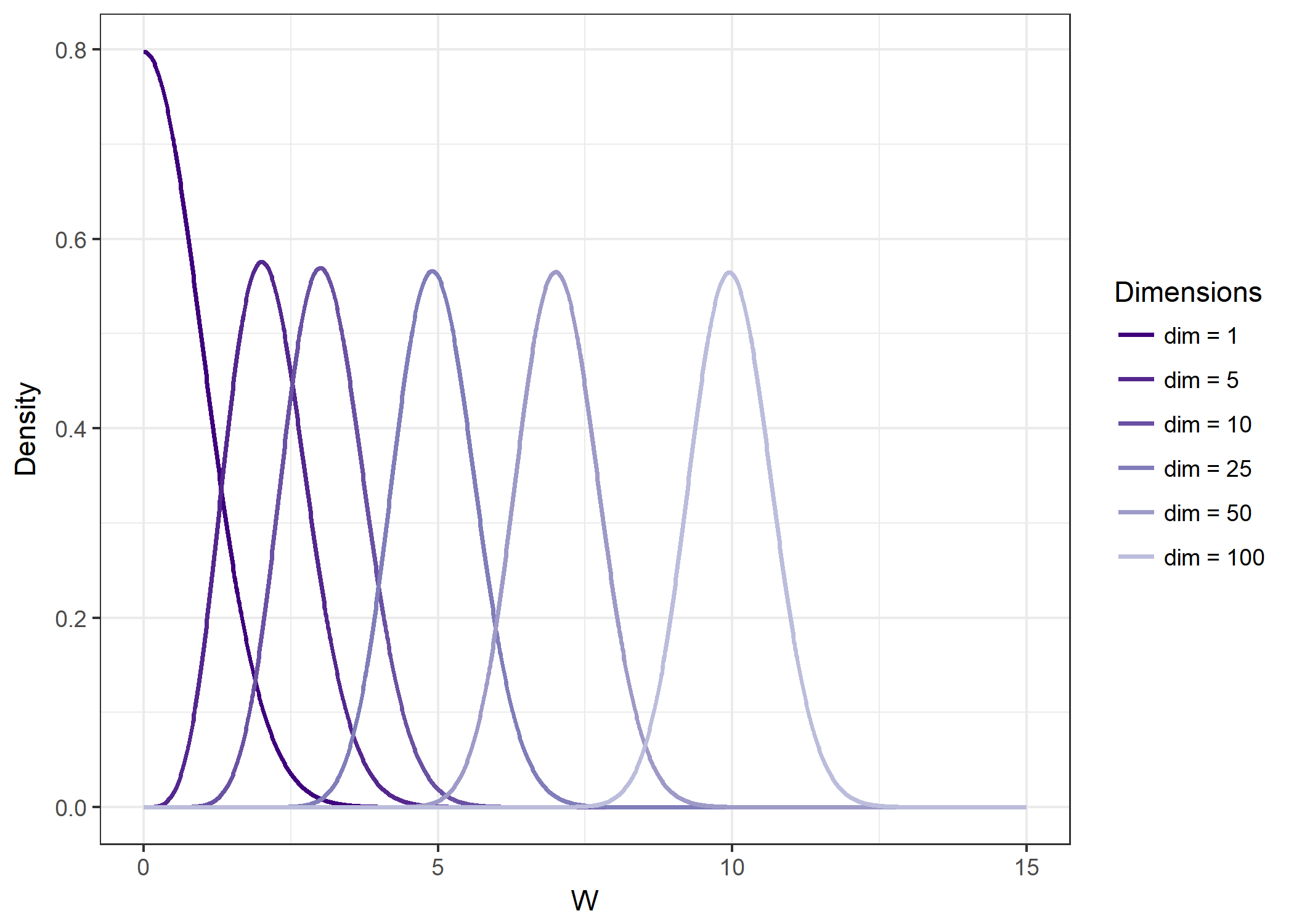

How can this be? A intuitive explanation is the following. Even though the density of the multivariate Normal distribution is concentrated near the origin, the probability mass is not only the density but the density times the volume over which we integrate the PDF. So, despite the fact that the density drops at an exponential rate from the origin outwards, the the volume that is located away from the origin grows even faster in high-dimensional spaces. The balance between these two tendenciesis found at the “shell,” which is where most of the probability is found.

The existence of such shell at which the probability mass is concentrated explains also why the random walk Metropolis algorithm tends to be relatively inefficient when sampling from high dimensional distributions. As shown in a previous post, the performance of the random walk Metropolis algorithm crucially depends on the step-size. Suppose that the probability mass is indeed concentrated in a thin shell somewhere distant from the origin. In this situation, using too large a stepsize will generate a lot of proposals that “jump away” from the region where the probability mass is concentrated (as the shell is “thin”), leading to high rejection rates and thus inefficient sampling; with small stepsizes, on the other hand, the algorithm will not be able to explore the entire distribution but rather stay in a small neighborhood, which leads to biased samples when the algorithm is not run sufficiently long. Yet, even for moderate step-sizes the Metropolis algorithm might have difficulties in exploring the “shell, “ and Hamiltonian Monte Carlo algorithms perform much better in these high-dimensional situations. This is because the reliance on Hamiltonian dynamics constraints the proposals to remain near the shell where the probability is concentrated. How much better HMC performs relative to Random-walk Metroplois depends on the application, however. For further details on the “curse of dimensionality” and MCMC methods, the 2017 STAN conference presentation by Michael Betancourt (starting approximately at 4:40) is very informative. Much of the intuition of this post comes from that video as well.