Slice Sampling
DISCLAIMER: This is a blog post from my graduate school years. The blog is no longer maintained and the material might include typos and errors.
The Fundamental Theorem
The main idea behind slice sampling is what Christian Robert and George Casella calls the Fundamental Theorem of Simulation in their book on Monte Carlo simulation. The theorem is based on the simple equation
\[\int_{0}^{p(x)} \,\text{d} y = p(x).\]Notice that the function we are integrating over is a constant function that is equal to one. To be more precise, it is the density $f(x,y) = \mathbb I_{\{(x,y): 0\le y\le p(x), x\in \mathcal X\}}(x,y)$, where $\mathbb I_{W}(w)$ is an indicator that is equal to one if $w\in W$ and zero otherwise, and where $\mathcal X$ is the support of a random variable $X$. That this function is a valid density is clear from the equation above since $\int_{\mathcal X} p(x) \text{d} x = 1$. Further, we see that the support of the joint density of $(X,Y)$ is just the set $\mathcal U = \{(x,y): 0\le y\le p(x), x\in \mathcal X\}$ which is the region under the density function of $X$. Thus, what the equation is saying is that if $(X,Y) \sim \text{Uniform}(\mathcal U)$, the marginal distribution of $X$ has the density $p$.
In practical terms, the Fundamental Theorem shows that we can obtain samples from the distribution $p$ by uniformly sampling under its curve. That is, if we sample the pair
\[(x,y) \sim \text{Uniform}(\mathcal U)\]and keep only the values of $x$, these will be samples from the desired distribution $p$. The variable $Y$ is thus an auxiliary variable, which is only introduced to make sampling possible but in which we have no substantive interest.
In fact, it turns out that we only need to know $p$ up to a constant of proportionality. To see this, let $p^\ast \propto p$ and define the set $\mathcal U^\ast = \{(x,y): 0 < y < p^\ast(x)\}$ (notice the $p^\ast$ in the definition). Then the uniform distribution of $(X,Y)$ over $\mathcal U^\ast$ is
\[p(x,y) = \begin{cases} k^{-1}, \qquad & \text{ if } 0 < y < p^\ast(x), \\ 0, &\text{otherwise}\end{cases}\]for some constant $k> 0$. And the marginal distribution of $X$ is
\[\int p(x,y)\,\text{d} y = \int_0^{p^\ast(x)} k^{-1} \,\text{d} y = k^{-1} p^\ast(x) \propto p(x)\]as desired. We also see immediately that $k = \int p^\ast(x) \,\text{d} x$ as the marginal density has to integrate to one.
The problem is that it is often difficult to create uniform draws from the region $\mathcal U$ or $\mathcal U^\ast$. A simple way to proceed is to use rejection sampling, which was discussed in more detail in a previous post.
Suppose we want to sample from a $p(x) \sim \text{Beta(2,5)}$ density. The density is defined over the interval $x\in (0,1)$ and its mode is attained at $x=0.2$ where the density evaluates as $p(x) \approx 2.46$. So, to create uniform draws from the region under the density $p(x)$, we might sample uniformly over the rectangle $\{(x,y) : 0 \le x\le 1 \text{ and } 0\le y\le 3\}$ and accept only those draws that satisfy the condition $y \le p(x).$ The accepted draws will be uniformly distributed over the desired set and, in this simple case, we know also that the acceptance rate will be approximately $1/3$ (as the area under $p$ is $1$ and the area of the rectangle is $3$).
An R code to show how this can be done is given below. Notice that the prop.fun function is the $\text{Beta(2,5)}$ density multiplied by a constant k. So, we are assuming that the distribution from which we want to sample is known up to a constant and that we can bound the function from above by a real number (which is $3k$ in this case). That is, while we want to sample from $p(x) \sim \text{Beta}(x\,\vert\,\alpha,\beta)$, what is available to us is only $p^\ast(x) = kp(x)$ and the information that $p\ast(x) < 3K$ for all $x\in \mathcal X$.
set.seed(123)
# set parameters

alpha = 2
beta = 5
n.sims = 6000

# some function proportional to beta(alpha, beta) density

k = runif(1) * 100
prop.fun = function(x) { k * dbeta(x, alpha, beta) }
message(paste0('Prop. const : ', round(k, 3)))
## Prop. const : 28.758
# sample uniformly over the rectangle [0, 1] X [0, 3 * k]

y = runif(n.sims, 0, 3 * k)
x = runif(n.sims, 0, 1)

# accept only values under the density

accept = (y <= prop.fun(x))
message(paste0('Acceptance rate : ', round(mean(accept), 3)))
## Acceptance rate : 0.335
The acceptance rate is close to $1/3$ (which it also should be by the Law of Large Numbers). Next we create a plot to illustrate how this sampling scheme works. The dots represent uniform draws over the rectangle $[0,1] \times [0, 3k]$, where accepted draws are plotted in blue and rejected draws in red. Further, we see that the distribution of the accepted $x$ values are approximately distributed as a $\text{Beta}(2,5)$ distribution, as desired.
# create grid

gd = seq(0, 1, .001)
# define colors for plotting

blue.3 = scales::alpha('blue', .3)
red.3 = scales::alpha('red', .3)
purple.5 = scales::alpha('purple', .5)

# parameters for plotting

par(mfrow = c(1, 2), mar = rep(2, 4))

# plot draws

plot(gd, prop.fun(gd), type = 'l', ylim = c(0,3 * k + 10),
     axes = T, frame.plot = F)
points(x[accept], y[accept], pch = '.', cex = 2, col = blue.3)
points(x[!accept], y[!accept], pch = '.', cex = 2, col = red.3)

# compare histogram of accepted draws with beta density

plot(gd, dbeta(gd, alpha, beta), type = 'l', ylim = c(0, 3),
     axes = T, frame.plot = F, col = 'grey50')
hist(x[accept], freq = F, add = T, breaks = 30,
     border = purple.5)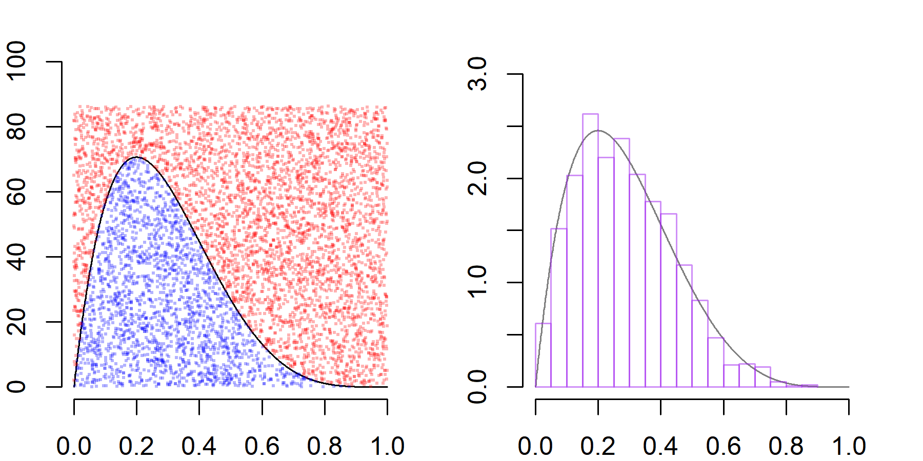
So it seems to work. However, this approach is not very efficient. After all, we are wasting $70\%$ of all simulations. Further, in other situations, we might not be able to bound the function form above nor might it be possible to find another function that dominates $p^\ast$ on $\mathcal X$. If $p^\ast$ is log-concave, adaptive rejection sampling might be a good way to obtain samples from $p$. Yet, suppose that $p^\ast$ does not satisfy this condition. A popular option in these scenarios, alongside the Metropolis-Hastings algorithm, is the slice sampler.
The Slice Sampler
The slice sampler can be thought of as a special case of the Gibbs sampler. Starting from an initial point $x_0$, we first uniformly draw $y_1$ from the interval $[0,p^\ast(x_0)]$. Thereafter, we draw $x_1$ from the horizontal “slice” at $y_1$, which is defined by the set $S_{y_1} = \{x: y_1 \le p^\ast(x)\}$. If $S_{y}$ is an interval, i.e., $S_y = [a,b]$ then the uniform distribution is characterized by the density
\[f(x) = \frac{1}{b-a} \mathbb I_{[a,b]}(x)\](Whether the interval is open or closed makes no difference, as density functions are only defined up to a set of probability zero). Similarly, in the case $S_{y_1}$ consists of multiple disjoint intervals, say $S_{y_1} = \bigcup_{k=1}^mI_k = \bigcup_{k=1}^m [a_k, b_k]$, the distribution is defined by
\[f(x) = \frac{1}{\mu(S_{y_1})}\mathbb I_{\{[a_1,b_1]\cup \cdots \cup [a_m,k_m]\}}(x),\]where $\mu(S_{y_1})$ denotes the “size” (the Lebesgue measure) of the set $S_{y_1}$ and is equal to $\mu(S_{y_1}) = \sum_{k=1}^m (b_k-a_k)$ since $I_k \cap I_{k’} = \varnothing$ for all $k\ne k’$.
While this formal definition might look complex, the idea is very simple (see the plot below). Starting from a point in the support of $X$, denoted in the code by x0 and represented by the blue vertical line, we draw y1 uniformly from the vertical interval between zero and the density. Next we consider the horizontal “slice” defined by y1, represented by the red horizontal line, and consider the set of all $x$ values “on” the slice, which is defined by the $x$ values for which the density is larger than y1.
# parameters for plotting

par(mfrow = c(1, 2), mar = rep(1, 4))

### Unimodal Beta(2,5) density ###


# plot density

plot(gd, dbeta(gd, alpha, beta), type = 'l', ylim = c(0, 3),
     axes = F, frame.plot = F, col = 'grey50')
abline(h = 0)

# starting value

x0 = .2
abline(v = x0, col = blue.3)

# sample y uniformly from [0, p(x0)]

y1 = runif(1, 0, dbeta(x0, alpha, beta))
abline(h = y1, col = red.3)

# find end-point of slice

m.roots = sort(
    rootSolve::uniroot.all(
        function(x) { dbeta(x, alpha, beta) - y1 },
        lower = 0,
        upper = 1
    )
)
# plot slice

segments(m.roots[1], y1, m.roots[2], y1, col = purple.5, lwd = 5)


### Bimodal mixture of Beta densities ###


# define density function

mix.beta = function(x) {
    .4 * dbeta(x, 2, 10) + .4 * dbeta(x, 10, 2) + .2 * dbeta(x, 5, 5)
}

# plot density

plot(gd, mix.beta(gd), type = 'l', ylim = c(0, 2), col = 'grey50',
     axes = F, frame.plot = F)
abline(h = 0)

# starting value

x0 = .2
abline(v = x0, col = blue.3)

# sample y uniformly from [0, p(x0)]

y1 = runif(1, 0, mix.beta(x0))
abline(h = y1, col = red.3)

# find end-points of slices

m.roots = sort(
    rootSolve::uniroot.all(
        function(x) { mix.beta(x) - y1 },
        lower = 0,
        upper = 1
    )
)

# draw slice

for (rr in 1:(length(m.roots) / 2)) {
    segments(m.roots[2 * rr - 1], y1, m.roots[2 * rr], y1,
             col = purple.5, lwd = 5)
}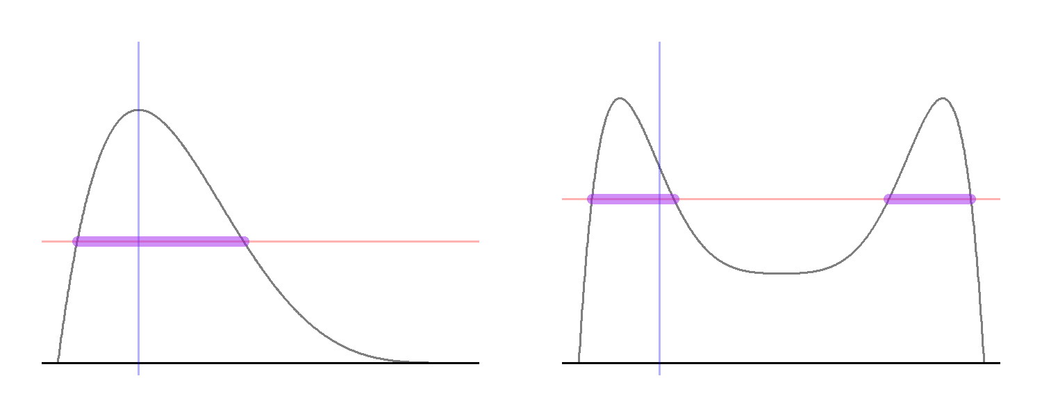
The plot on the right-hand side shows why it might not possible to represent the horizontal slice as a single interval. Here, the target density is bimodal so that, for some $y$ values, the horizontal slice consists of two disjoint intervals rather than one. Yet, the logic remains the same: we draw a horizontal line at the sampled $y$-value and sample uniformly from all the $x$-values that are in the set $\{x: y\le p^\ast(x)\}$.
Notice that both of the distributions from which we are sampling are conditional distributions and that we accept the samples with probability one, which shows that the slice sampler can be thought of as a particular case of Gibbs sampling. Further, it turns out this sampling scheme let’s our target, i.e., the uniform distribution over the set $\mathcal U = \{(x,y): 0 \le y \le p^\ast(x)\}$, invariant.
Illustrating this point is straightforward. First, given that we start from $y^{(s-1)}$, the distribution of $x^{(s)}$ depends only on $y^{(s-1)}$ and that of $y^{(s)}$ only on $x^{(s)}$. Hence, the sampling scheme indeed forms a Markov chain. We have to show that the Markov transitions leave the joint distribution $p(x,y)$ and, thus, marginal distribution $p(x)$, invariant. Let us abuse notation a little bit and denote all realized values as well as random variables with lower-case letters. Suppose that $x_t \sim p$. Then, $y_{t+1}\, \vert \, x_{t} \sim \text{Uniform}(0,p^\ast(x_t))$ and the joint distribution of $(x_t, y_{t+1})$ is
\[\begin{aligned} p(x_{t}, y_{t+1}) &= p(x_{t})p(y_{t+1}\, \vert \, x_{t}) \\ &= k^{-1} p^\ast(x_t) \frac{\mathbb I_{\{0\le y_{t+1}\le p^\ast(x_t)\}}(y_{t+1})}{p^\ast(x_t)} \\ &\propto \mathbb I_{\{ 0 \le y_{t+1}\le p^\ast(x_t)\}}(x_t, y_{t+1}). \end{aligned}\]Next, the conditional distribution of $x_{t+1}$ depends only on $y_{t+1}$ and is uniform over the slice $S_{y_{t+1}} = \{x: y_{t+1}\le p^\ast(x)\}$. So,
\[\begin{aligned} p(y_{t+1}, x_t, x_{t+1}) &= p( y_{t+1}, x_t)p( x_{t+1}\, \vert \, y_{t+1}, x_t) = p( y_{t+1}, x_t)p( x_{t+1}\, \vert \, y_{t+1}) \\ &\propto \mathbb I_{\{0 \le y_{t+1}\le p^\ast(x_t)\}}(x_t,y_{t+1}) \frac{\mathbb I_{\{y_{t+1}\le p^\ast(x_{t+1})\}}(x_{t+1})}{\mu(S_{y_{t+1}})} \end{aligned}\]To obtain the distribution of $(y_{t+1}, x_{t+1})$, we have to integrate $x_t$ out. The only term that depends on $x_t$ is the indicator function $\mathbb I_{\{0 \le y_{t+1}\le p^\ast(x_t)\}}(x_t,y_{t+1})$, and
\[\begin{aligned} \int \mathbb I_{\{0 \le y_{t+1}\le p^\ast(x_t)\}}(x_t,y_{t+1})\,\text{d} x_t &= \mathbb I_{\{0\le y_{t+1}\}}(y_{t+1})\int \mathbb I_{\{y_{t+1} \le p^\ast(x_t)\}}(x_t) \,\text{d} x_t \\ &= \mathbb I_{\{0\le y_{t+1}\}}(y_{t+1}) \mu(\{x: y_{t+1} \le p^\ast(x)\}) \\ &= \mathbb I_{\{0\le y_{t+1}\}}(y_{t+1}) \mu(S_{y_{t+1}}) \end{aligned}\]It follows that
\[\begin{aligned} p(x_{t+1},y_{t+1} ) &= \int p(y_{t+1}, x_t, x_{t+1})\,\text{d} x_t\\ &\propto \frac{\mathbb I_{\{y_{t+1}\le p^\ast(x_{t+1})\}}(x_{t+1})}{\mu(S_{y_{t+1}})}\int \mathbb I_{\{0 \le y_{t+1}\le p^\ast(x_t)\}}(x_t,y_{t+1}) \,\text{d} x_t \\ &= \frac{\mathbb I_{\{y_{t+1}\le p^\ast(x_{t+1})\}}(x_{t+1})}{\mu(S_{y_{t+1}})}\mathbb I_{\{0\le y_{t+1}\}}(y_{t+1}) \mu(S_{y_{t+1}})\\ &= \mathbb I_{\{y_{t+1}\le p^\ast(x_{t+1})\}}(x_{t+1})\mathbb I_{\{0\le y_{t+1}\}}(y_{t+1}) \\ &= \mathbb I_{\{0\le y_{t+1}\le p^\ast(x_{t+1})\}}(x_{t+1}, y_{t+1}) \end{aligned}\]which is the same distribution as that of $(x_t,y_{t+1})$. Hence, if $x_t$ is drawn from $p$, then so will be $x_{t+1}$, showing that the slice sampling scheme leaves the target distribution invariant.
Stepping Out and Shrinkage
The real difficulty lies in the implementation of the slice sampler. Sampling $y \sim [0,p^\ast(x)]$ is easy; the major challenge is how to sample uniformly from the horizontal slice at $y$. If the set $S_y$ can be determined analytically, which amounts to finding the solutions to $y = f(x)$, sampling from $S_y$ is straightforward. Yet, this is often not possible, so let us assume that an analytical solution does not exist. Next, suppose that the support of $X$ is bounded, $\mathcal X = [a,b]$. Then, we can use rejection sampling and draw $\text{Uniform}(a,b)$ until we get a sample that is contained in the slice. As we’ve examined above, the accepted draws will be uniform on $S_{y}$, so the algorithm will be correct. But,this approach will be extremely inefficient in the case $S_{y}$ is much smaller a set than $\mathcal X$. Further, this method does not help us with densities that have unbounded support.
In a great and accessible-even-to-sociologists paper, Radford Neal proposed two methods to sample from $S_y$ efficiently: the “stepping out” method and the “doubling” method. Here, we’ll be concerned with former. To use the stepping-out algorithm, we need to define a tuning parameter $w$, which should reflect our estimate of the typical size of the slice. Let us first assume that the distribution $p$ is unimodal, so that we don’t have to deal with slices that consists of multiple intervals and we can write $S_y = \{x: l \le x \le u\}$.
We first generate a random interval of size $w$ that contains the current $x$-value. Let us denote this interval by $I_x=[a,b]$. If $a < \inf \mathcal X$ then set $a := \inf \mathcal X$ and analogously set $b := \sup \mathcal X$ if $b > \sup \mathcal X$. Now, suppose that $I_x \subseteq S_y$, implying that $l \le a \le x \le b \le u$. As we want a uniform draw from $[l,u]$, the interval $I_x[a,b]$ will be too short. So, we expand $I_x$ by extending it below and above by an amount of $w$, such that the resulting interval looks like $[a-w, b+w]$. If $a-w \le l$, then we fix the lower-limit of our interval there; if not, we keep expanding until $a - M w \le l$ for some positive integer $M$. We do the same for the upper-limit of $I_x$, this time increasing the limit by an amount of $w$ until we have $b + M’ w \ge u$ for some positive integer $M’$. The end result of this process is a new interval $I_x^\star$ that contains $S_y$. This is the “stepping out” process of the algorithm. Clearly, if both end-points of the initial interval are already outside of the slice, we have $I_x = I_x^\star$.
After finding an interval $I_x^\star$ that contains $S_y$, we can use rejection sampling to obtain a uniform draw from $S_y$. That is, sample $x^\ast \sim I_x^\star$ and accept $x^\ast$ as a new sample of $X$ if $y \le p^\ast(x^\ast)$; otherwise, reject $x^\ast$ and sample again. As $S_y \subset I_x^\star \subset \mathcal X$ this approach will be more efficient than directly drawing $x^\ast \sim \text{Uniform}(\mathcal X)$. The figure below shows the process of “stepping out” in a case where $S_y$ consists of multiple intervals. The $\times$ in the first row shows the current $x$-value and the thick purple lines represent the slice $S_y$. The next line shows the initial interval of size $w$, which is chosen intentionally to be smaller than the size of the slice. As both of the endpoints lie inside of the slice, we keep expanding both sides until we step out of the slice, which is shown in the third row. Then we sample uniformly over the created interval until we get a $x$-value that lines in the slice, which is presented in the last row of the plot.
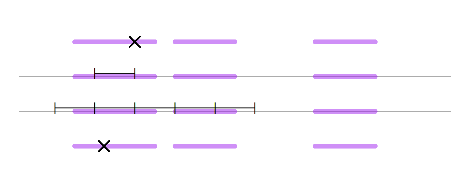
But there is an additional trick that Neal introduces. Namely, suppose that we’ve sampled $x^\ast$ from the interval $I_x^\star$ but that $p^\ast(x^\ast) < y$. That is, the proposal lies outside of the slice, $x^\ast\in I_x^\star \setminus S_y$. Then we can “shrink” $I_x^\star$ to a new interval $I_x^\ast$ in the following way. If $x^\ast < a$, then set $a^\ast := x^\ast$; if $x^\ast > b$, then set $b^\ast := x^\ast$. As it is ensured that $S_y\subset I_x^\ast \subset I_x^\star$, every failed draw will increase the probability that the next draw is in the slice.
The figure above also points out some theoretical complexities that arise when the target distribution $p$ is multimodal. With the current window size and this specific horizontal slice, the probability of sampling a new value from the right-most interval is zero. So, we would not be able to take a uniform sample from $S_y$. Notice, however, that this might not be true for the slices defined at other $y$-values. In the beta-mixture distribution examined above, for example, the horizontal slice will contain almost all points of $\mathcal X$ if the last sampled value of $y$ is sufficiently small. A quite intuitive proof that the slice sampler using all of the intermediate steps—creating the initial window, stepping out, and shrinking—works for a large family of distributions, including multimodal ones, can be found in Neal’s paper mentioned above. Of course, if there exists an interval $I \subset \mathcal X$ for which $\vert I\vert > w$ and $f(x) = 0$ for all $x \in I$, the slice sampler will not be able to jump from one side of the interval to the other side. Except for such pathological cases, however, there will be always a non-zero probability for the sampler to move from the current $x_t$ to any other point in $\mathcal X$ by hitting the right slice, so to say.
Implementation
The slice sampler is easy to code up and is very general. All we need to specify is a function $p^\ast$ that is proportional to the target, the window size $w$, an initial value for $x$, and the number of simulations we desire. Below is a function that implements the slice sampler. Two small notes. First, in the shrinking procedure, we check whether x > x.old, where x is the new proposal and x.old is the old value of $x$ rather than checking whether the proposal is greater or smaller than the upper and lower limit of our current interval, $[l,u]$. This code works because the old $x$-value is always a member of the slice $S_y$. Hence, if $x^\ast > x$ but $x^\ast \notin S_y$, this implies that $x^\ast$ must be greater than $u$. Similarly, if $x^\ast < x \text{ and } x^\ast \notin S_y$, then $x^\ast < l$. Second, in any real implementation of the sampler, it will be better to work on the log-scale for numerical stability. For this toy example, we just work directly on the probability scale.
SliceSampler = function(x, pstar, w, n.sims) {

    # define function to check whether proposal is in slice

    in.slice = function(x, y) { y <= pstar(x) }

    # container for sampled values

    sims = matrix(NA, n.sims, 2)

    for (s in 1:n.sims) {

        ### sample y ###


        y = runif(1, 0, pstar(x))


        ### sample x ###


        # initial window


        l = x - w * runif(1)
        u = l + w

        # expand lower-limit if necessary


        l.in = in.slice(l, y)
        if (l.in) {

            while (l.in) {

                l = l - w

                # check whether lower bound is hit

                if (l < 0) {

                    l = 0
                    break

                }

                l.in = in.slice(l, y)

            }

        }

        # expand upper-limit if necessary


        u.in = in.slice(u, y)
        if (u.in) {

            while (u.in) {

                u = u + w

                # check whether upper bound is hit

                if (u > 1) {

                    u = 1
                    break
                }

                u.in = in.slice(u, y)

            }

        }

        # sample x from y-slice and shrink


        x.old = x
        x.in = FALSE

        while (!x.in) {

            # sample x

            x = runif(1, l, u)

            # check whether x is in slice

            x.in = in.slice(x, y)

            # shrink interval

            if (x > x.old) {

                u = x

            } else {

                l = x

            }

        }

        # store samples

        sims[s, 1] = x
        sims[s, 2] = y

    }

    return(sims)

}
Next, we specify our inputs and run the sampler.
# number of simulation draws to take

n.sims = 30000
# initial value of x

x.init = .5
# old beta(2, 5) density multiplied by constant

beta.prop = function(x) { k * dbeta(x, alpha, beta) }
# new mixture distribution, with smaller density in the middle

mix.beta = function(x) {
  .45 * dbeta(x, 2, 10) + .45 * dbeta(x, 10, 2) + .1 * dbeta(x, 3, 3)
}
# window size

w = .2

# start sampling

start.time = Sys.time()
slice.samps.beta = SliceSampler(
    x.init,
    beta.prop,
    w,
    n.sims)
print(Sys.time() - start.time)
## Time difference of 2.383635 secs
start.time = Sys.time()
slice.samps.mix = SliceSampler(
    x.init,
    mix.beta,
    w,
    n.sims)
print(Sys.time() - start.time)
## Time difference of 2.859364 secs
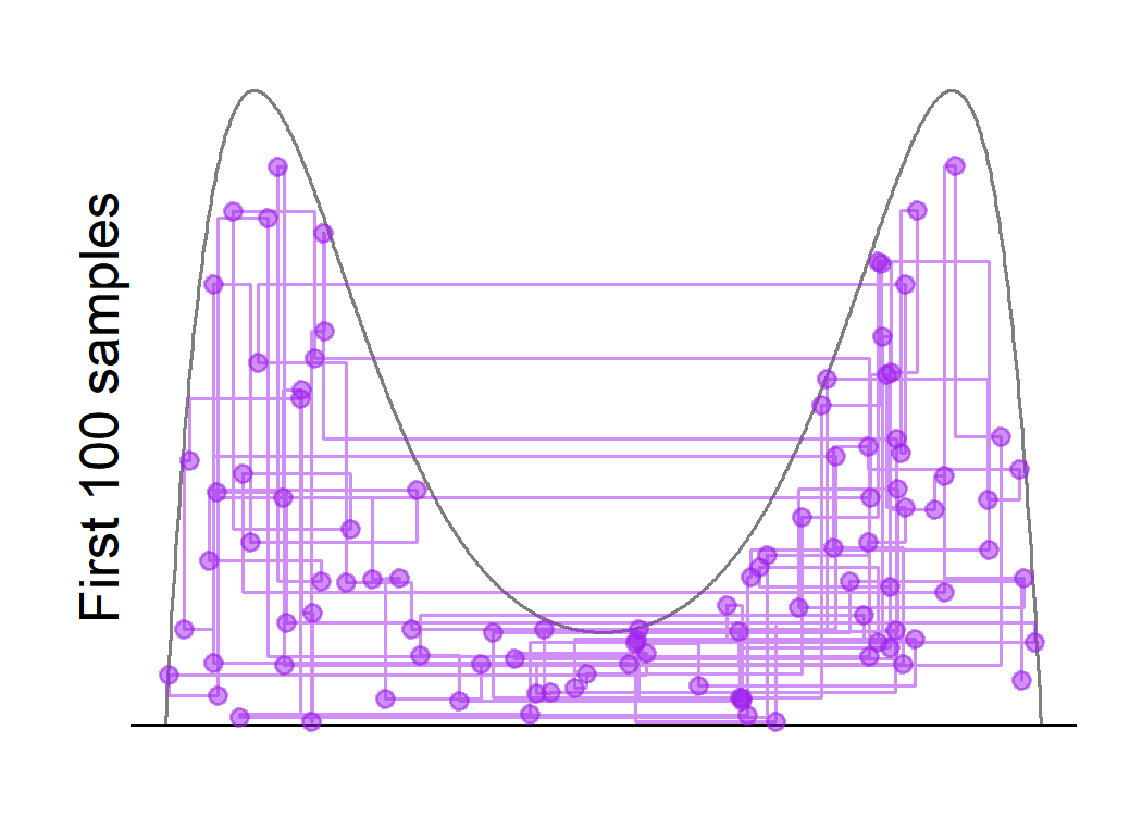
The sampler runs quite fast, generating n.sim = 30,000 samples in less than three seconds. We might again plot the behavior of the sampler:
# function for plotting path of sampler

gen.path = function(sims, n.draw) {

    if (nrow(sims) > n.draw) {

        z = sims[1:(n.draw + 1), ]

    } else {

        z = rbind(sims, sims[nrow(sims), ])

    }


    path.mat = lapply(1:n.draw, function(w) {
        z1 = z2 = z[w, ]
        z2[2] = z[w + 1, 2]
        return(rbind(z1, z2))
    })

    do.call('rbind', path.mat)

}

# subsample first 100 draws and generate path


n.draw = 100
path.mat.beta = gen.path(slice.samps.beta, n.draw)
path.mat.mix = gen.path(slice.samps.mix, n.draw)

# plot samples

par(mfrow = c(2, 2), mar = c(1, 2, 1, 1))
plot(gd, beta.prop(gd), type = 'l',
     axes = F, frame.plot = F, col = 'grey50',
     ylab = '')
abline(h = 0)
lines(path.mat.beta, col = purple.5)
points(slice.samps.beta[1:n.draw, ], col = purple.5,
       pch = 19, cex = .75)
mtext(paste0('First ', n.draw, ' samples'), outer = F, side = 2)

plot(gd, mix.beta(gd), type = 'l',
     axes = F, frame.plot = F, col = 'grey50')
abline(h = 0)
lines(path.mat.mix, type = 'l', col = purple.5)
points(slice.samps.mix[1:n.draw, ], col = purple.5,
       pch = 19, cex = .75)

plot(gd, dbeta(gd, alpha, beta), type = 'l',
     axes = F, frame.plot = F, col = 'grey50',
     ylab = '')
abline(h = 0)
hist(slice.samps.beta[ , 1], border = purple.5,
     fill ='white', freq = F, add = T, breaks = 100)
mtext(paste0('All samples'), outer = F, side = 2)

plot(gd, mix.beta(gd), type = 'l',
     axes = F, frame.plot = F, col = 'grey50')
abline(h = 0)
hist(slice.samps.mix[ , 1], border = purple.5,
     fill ='white', freq = F, add = T, breaks = 100)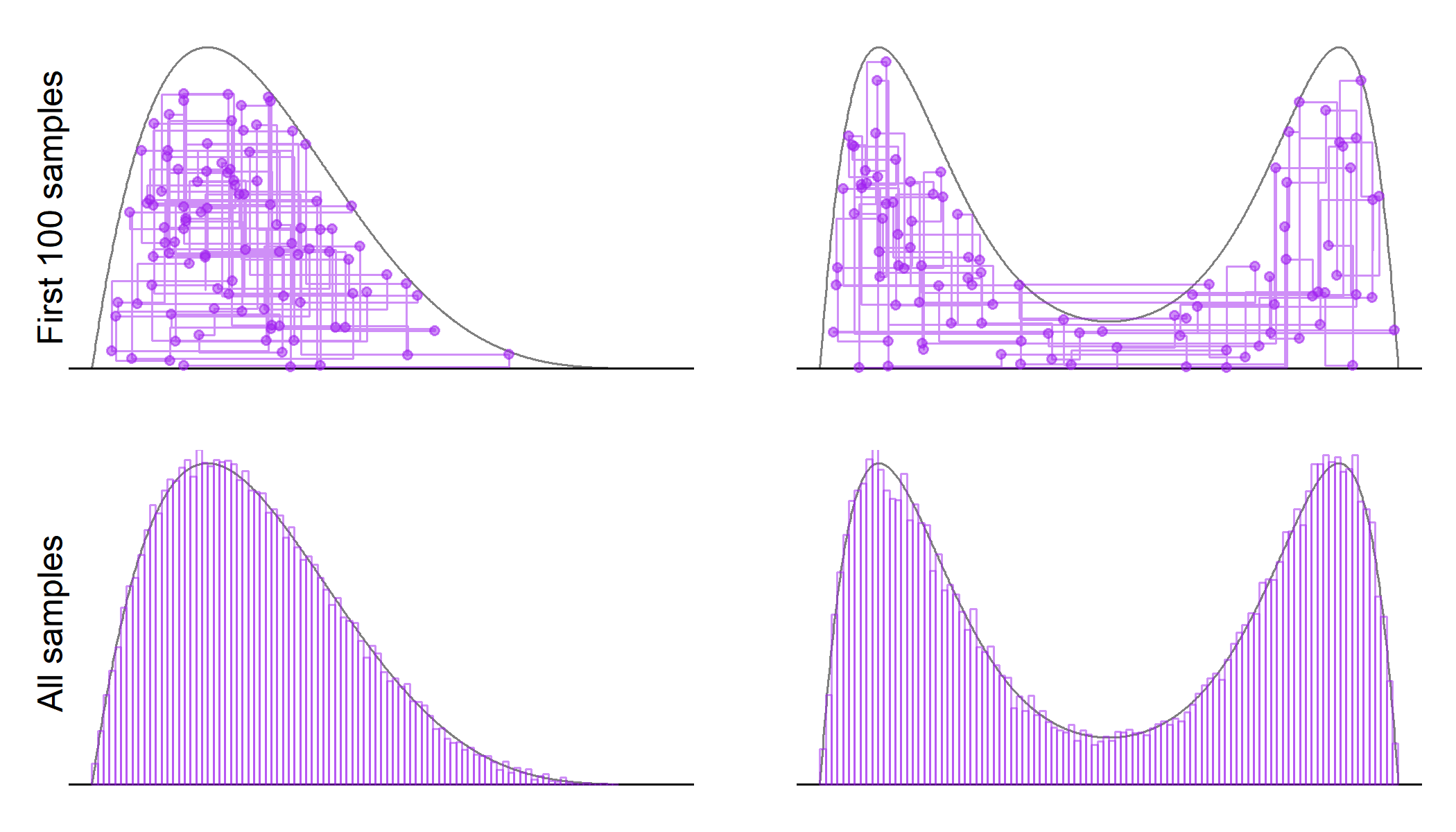
The lines in the first row show the trajectory of the sampler, while the second row shows the histogram of the marginal distribution of $X$ overlaid on the true target densities. The trajectory looks a lot like the Gibbs sampler, which is also expected. The points denote the sampled values of the $(x,y)$ pair. Notice that small values of the auxiliary variable $y$ are sampled frequently enough for the sampler to move between the two modes in the bimodal distribution. However, it is also clear that once the sampler enters one of the modes, it will stay there for a while before moving to the other mode. This behavior of the sampler will create more autocorrelation between subsequent samples for the bimodal distribution. This is also reflected in the effective sample size, which is about one-fifth for the bimodal distribution when compared to the unimodal one
esize = c(round(coda::effectiveSize(slice.samps.beta[ , 1]), 2),
          round(coda::effectiveSize(slice.samps.mix[ , 1]), 2))
names(esize) = c('Unimodal', 'Bimodal')
print(esize)
## Unimodal Bimodal
## 22910.93 4051.98
or in the diagnostics plots shown below:
# plot autocorrelations and traceplot

par(mfrow = c(3, 2), mar=c(2, 4, 2, 1))
blue.7 = scales::alpha('blue', .7)

coda::autocorr.plot(slice.samps.beta[ , 1],
              auto.layout = F, col = 'blue',
              main = 'Beta(2,5) Density')
coda::autocorr.plot(slice.samps.mix[ , 1],
              auto.layout = F, col = 'blue',
              main = 'Mixture of Beta Densities')
plot(slice.samps.beta[1:n.draw, 1], ylim = c(0, 1),
     type = 'l', col = 'blue',
     ylab = 'First 100 Iterations')
plot(slice.samps.mix[1:n.draw, 1], ylim = c(0, 1),
     type = 'l', col = 'blue',
     ylab = 'First 100 Iterations')
plot(slice.samps.beta[ , 1],
          ylim = c(0, 1),
          col = blue.7,
          pch = 16, cex = .1,
     ylab = 'All Iterations')
plot(slice.samps.mix[ , 1], ylim = c(0, 1),
     col = blue.7, pch = 16, cex = .1,
     ylab = 'All Iterations')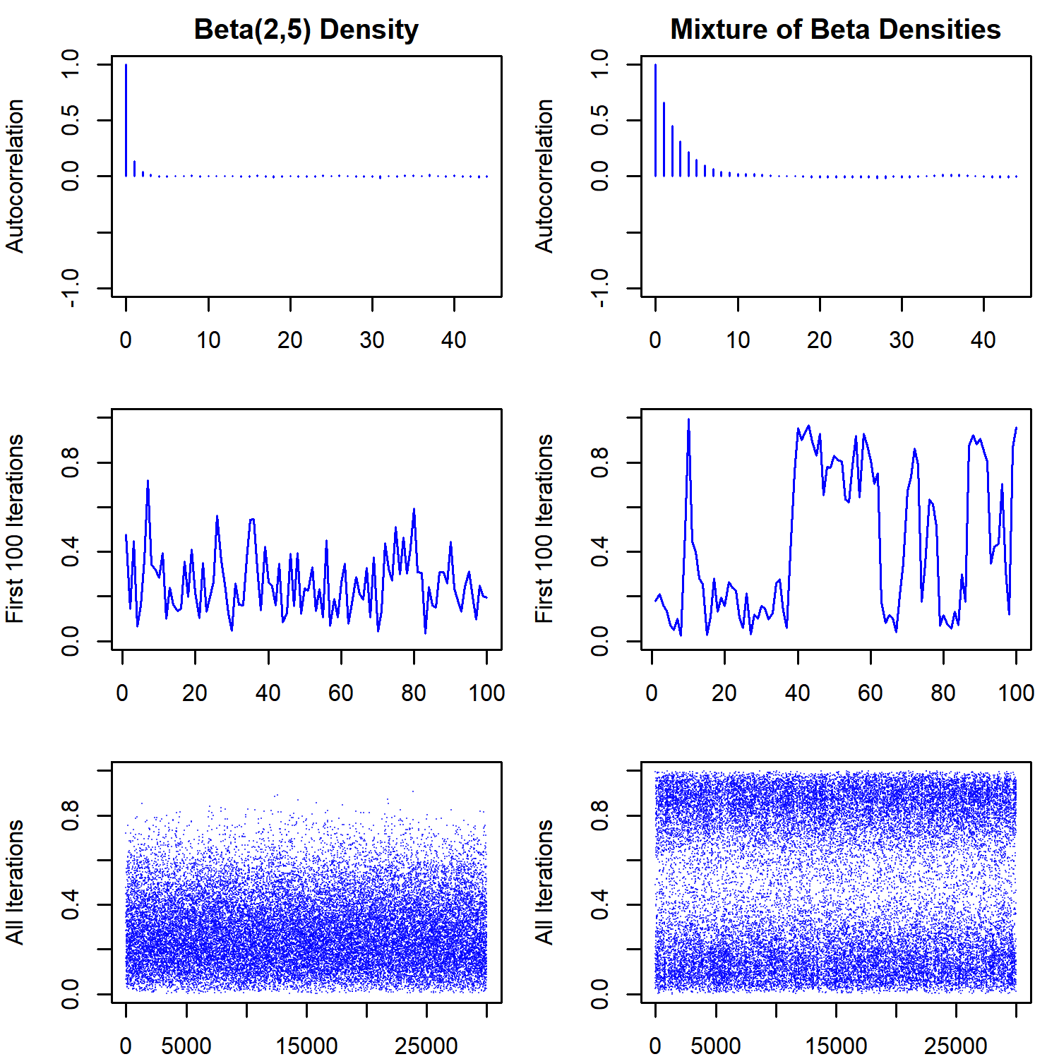
Notice that the traceplot for the bimodal distribution looks a lot like traceplot where label switching is occurring. This shows that one has to be careful with models where the likelihood is not identified (in the sense that different parameter values can lead to the same likelihood). Multimodality of the posterior might be a symptom of the unidentified likelihood, the posterior distribution itself, or both.
One interesting question that arises is what would happen if we increase the window-size. For example, specifying the window size to be $w = 1$ will make it quite likely that the first proposal for the next move will be uniformly distributed on $[0,1]$ regardless of the current state, although the shrinkage procedure will generate more accepted states that are close to the current value. This might increase the effective sample size by reducing the autocorrelations between subsequent samples.
start.time = Sys.time()
slice.samps.mix.2 = SliceSampler(
    x.init,
    mix.beta,
    1,
    n.sims)
print(Sys.time() - start.time)
## Time difference of 2.858363 secs
n.draw = 100
path.mat.mix.2 = gen.path(slice.samps.mix.2, n.draw)

# plot samples

par(mfrow = c(1, 1), mar = c(1, 2, 1, 1))
plot(gd, mix.beta(gd), type = 'l',
     axes = F, frame.plot = F, col = 'grey50')
abline(h = 0)
lines(path.mat.mix.2, type = 'l', col = purple.5)
points(slice.samps.mix.2[1:n.draw, ], col = purple.5, pch = 19, cex = .75)
mtext(paste0('First ', n.draw, ' samples'), outer = F, side = 2)

print(round(coda::effectiveSize(slice.samps.mix.2[ , 1]), 2))
## var1
## 11395.38
We see that the sampler is now able to jump from one mode to the other, even for large values of $y$. Also, the effective sample size is about two times of that in the last run, although the running time is increased as well.
This raises the question of how to choose $w$, the window size. One way to deal with the problem is to let the sampler run for a short time in order to obtain an estimate of the typical slice size and to use it in the subsequent sampling. Notice that this might run into problems when we have multimodal distributions, as the estimated window size will often not span across all of the modes.
As I was planning on using the slice sampler in a project of mine anyways, I’ve coded up a Rcpp function to implement it (disclaimer: I’m still in the process of learning how to code in C/C++). The code is slightly more evolved with a few additional features. For example, now we are working on the log-probability scale for numerical stability and allow the specification of upper and lower bounds on the support of the target density. We also have to feed into the slice_sampler function a pointer to an externally defined function, so that we can apply it to different target densities. Lastly, note that the function defined in the last chunk of code is simply there to call the function from R, which will not be necessary when we use the slice sampler as a step in a larger Gibbs sampling scheme. The wbar object will calculate the running average of the window sizes over the iterations, which is printed out at the end of the sampling procedure.
#include <Rcpp.h>
using namespace Rcpp;

//' Function Proportional to Target Density (on the log-scale)

//'

//' The good-old Beta(2, 5) Density multiplied by 5 on the log-scale

//'

//' @param x point at which target should be evaluated

//' @return log-density of target (plus a constant)


inline double log_p(double x) {

    return log(5.0) + R::dbeta(x, 2.0, 5.0, true) ;

}

//' In-slice Check

//'

//' Function to check whether sampled proposal is element of the slice

//'

//' @param log_p pointer to the target log-density (plus a constant)

//' @param x     proposal in the rejection sampling step

//' @param log_y logarithm of the sampled y-value in current slice

//'              sampling step

//' @return      true if proposal is in the slice and false otherwise


inline bool check_slice(double (*log_p)(double x),
                 double x,
                 double log_y)
{

    return log_y <= log_p(x);

}

//' Univariate Slice Sampler

//'

//' Samples from the distribution proportional to \code{pstar} using

//' slice sampling

//'

//' @param x          initial value to start sampling

//' @param log_p      pointer to the target log-density

//' @param ub         upper bound of support

//' @param lb         lower bound of support

//' @param w          window size to use

//' @param sims       number of samples to take

//' @param maxit      maximum number of iterations during sampling

//' @param print_wbar whether to print the avg. window size

//' @return           a length-\code{sims} vector of samples from

//'                   the target distribution


NumericVector slice_sampler(
        double x,
        double (*log_fun)(double x),
        double w,
        double lb,
        double ub,
        int sims,
        int maxit,
        bool print_wbar = false)
{

    NumericVector res(sims);
    double log_y(0.0), l(0.0), u(0.0), x_old(0.0), wbar(0.0);
    int nn(0L), ii;
    bool inslice(false);
    NumericVector::iterator s;

    // start sampling //


    for (s = res.begin(); s != res.end(); ++s) {

        // sample y //

        log_y = log_p(x) + log(R::runif(0.0, 1.0));

        // sample x ...


        // initial window

        l = x - R::runif(0.0, w);
        u = l + w;

        // expand lower-limit if necessary


        if (check_slice(log_p, x, log_y)) {

            for (ii = 0; ii < maxit; ++ii) {

                l = l - w;

                // check whether lower bound is hit

                if (l < lb) {

                    l = lb;
                    break;

                }

                if (!check_slice(log_p, l, log_y))
                    break;

            }

        }

        // expand upper-limit if necessary


        if (check_slice(log_p, u, log_y)) {

            for(ii = 0; ii < maxit; ++ii) {

                u = u + w;

                //check whether upper bound is hit

                if (u > ub) {

                    u = ub;
                    break;
                }

                if (!check_slice(log_p, u, log_y))
                    break;

            }

        }

        // sample x from y-slice and shrink


        x_old = x;

        for (ii = 0; ii < maxit; ++ii) {

            // sample x

            x = R::runif(l, u);

            // check whether x is in slice

            if (check_slice(log_p, x, log_y))
                break;

            // shrink interval

            if (x > x_old) {

                u = x;

            } else {

                l = x;

            }

        }

        // update average window size

        if (print_wbar) {
            ++nn;
            wbar = (nn * wbar + (u - l)) / (nn + 1.0);
        }

        // store new x

        *s = x;

    }

    if (print_wbar)
        Rcout << "Avg. window size : " << wbar << std::endl;

    return res;

}

//' Slice Sampler (to be exported)

//'

//' This is just a wraper to call the slice sampler from R


//[[Rcpp::export()]]

NumericVector run_slice_beta(
        double x,
        double w,
        double lb,
        double ub,
        int sims,
        int maxit,
        bool print_wbar) {

    return slice_sampler(
        x,
        log_p,
        w,
        lb,
        ub,
        sims,
        maxit,
        print_wbar);
}
We might check whether the code works properly by, first, sourcing the C++ function into our R environment and, then, running a toy example. The small C++ code can be sourced by running
Rcpp::sourceCpp('name_of_cpp_fun.cpp')We might compare the results of our new function with our old sampler:
n.sims = 30000
old.beta = function(x) 5 * dbeta(x, alpha, beta)

start.time = Sys.time()
old.beta.samps = SliceSampler(
    x.init,
    old.beta,
    w,
    n.sims)
print(Sys.time() - start.time)
## Time difference of 2.530552 secs
start.time = Sys.time()
new.beta.samps = run_slice_beta(
    x = x.init,
    w = w,
    lb = 0,
    ub = 1,
    sims = n.sims,
    maxit = 100,
    print_wbar = T)
print(Sys.time() - start.time)
## Avg. window size : 0.708174
## Time difference of 0.07395816 secs
par(mfrow = c(1,3))
qqplot(old.beta.samps[,1], new.beta.samps, col = red.3,
       xlab = 'R', ylab = 'Rcpp')
abline(a = 0, b = 1, col = blue.7)
qqplot(y = new.beta.samps, rbeta(n.sims, alpha, beta), col = red.3,
       xlab = 'Sims', ylab = 'Rcpp')
abline(a = 0, b = 1, col = blue.7)
qqplot(y = new.beta.samps, rbeta(n.sims, alpha, beta), col = red.3,
       xlab = 'Sims', ylab = 'R')
abline(a = 0, b = 1, col = blue.7)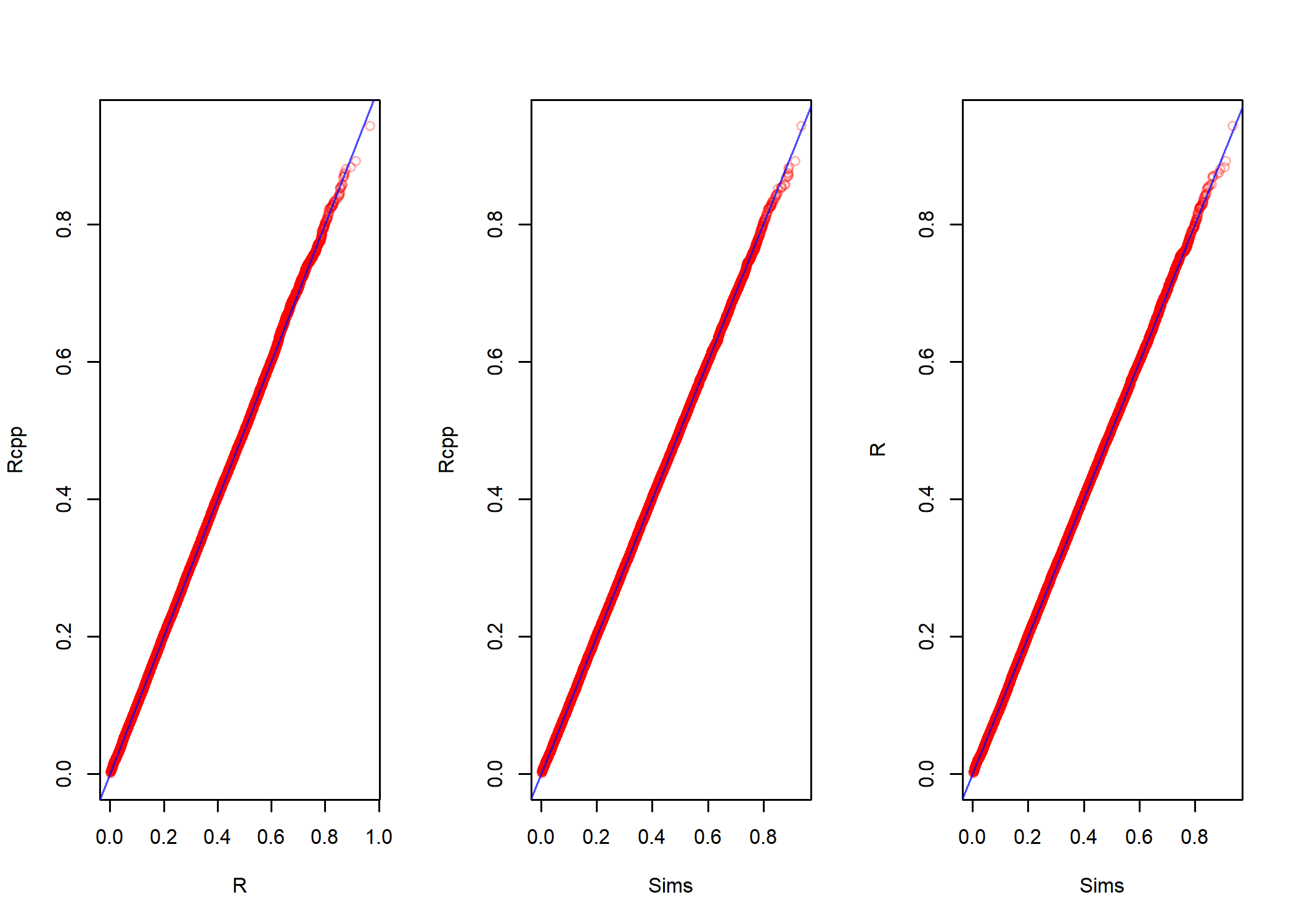
So, it seems to work and that the average size of the typical slice is about $0.7$. Using this as our estimate, we might run the sampler again and check how much it improves the algorithm. We set the number of samples to take to n.sims = 10000 and run the sampler with window size specified to w = c(.1, .4, .7, 1.0). This is repeated times = 500 times and the elapsed time is compared.
n.sims = 5000
microbenchmark::microbenchmark(
    w1 = run_slice_beta(
            x = x.init,
            w = .1,
            lb = 0,
            ub = 1,
            sims = n.sims,
            maxit = 100,
            print_wbar = F),
    w3 = run_slice_beta(
            x = x.init,
            w = .3,
            lb = 0,
            ub = 1,
            sims = n.sims,
            maxit = 100,
            print_wbar = F),
    w7 = run_slice_beta(
            x = x.init,
            w = .7,
            lb = 0,
            ub = 1,
            sims = n.sims,
            maxit = 100,
            print_wbar = F),
    w10 = run_slice_beta(
            x = x.init,
            w = 1,
            lb = 0,
            ub = 1,
            sims = n.sims,
            maxit = 100,
            print_wbar = F),
    times = 500
)
## Unit: milliseconds
## expr min lq mean median uq max neval cld
## w1 18.94636 21.38532 26.26502 23.45658 26.94156 141.39817 500 c
## w3 12.16383 13.88590 16.98465 15.35941 17.27092 175.51071 500 b
## w7 10.59527 12.06387 14.63524 13.67416 15.84515 79.26169 500 a
## w10 10.12671 11.48353 14.39788 12.68839 15.00688 103.25333 500 a
We see that the efficiency of the sampler is quite robust to overspecifying the width of the window size thanks to the “shrinkage” step (as also argued by Neal). Hence, if we are not certain about how large the window should be, it seems to be a sensible choice to set it a little bit larger than our best estimate. This will also reduce the autocorrelation across subsequent samples if the target density is multimodal by letting the sampler jump from one mode to the other in one step as we’ve seen above (if all the modes are within the reach of the window, of course).