Maximum Simulated Likelihood
DISCLAIMER: This is a blog post from my graduate school years. The blog is no longer maintained and the material might include typos and errors.
In preparation for a new project, I am currently trying out different methods to estimate the parameters of a model I have in my mind. It turns out that it is always some kind of integral that greatly complicates estimation. For example, in Bayesian statistics, the normalizing constant is defined in terms of an integral (or a sum); when using marginal likelihood methods, the marginalization is also done by integration, when the parameters are continuous. So, the evaluation of that integral, or side-stepping it, becomes always a problem.
In maximum likelihood estimation of multilevel models, a common way to go is using quadrature. This approach is quite efficient if the number of random components in the model is small, and by small I mean really small, such as one or two. With more random components, approximations using quadrature can be computationally more demanding than other approaches. One alternative approach to estimate these models is to use Monte Carlo simulation.
For example, consider the following simple multilevel model,
\[\begin{aligned} Y_{ij} &= \mu_\theta + \theta_i + \epsilon_{ij} \\ \theta_i &\sim \text{Normal}(0, \sigma_\theta) \\ \epsilon_{ij} &\sim \text{Normal}(0,\sigma_\epsilon) \end{aligned}\]where the subscript $i$ stands for groups and $j$ for individuals in the groups. The DAG of the data-generating process is shown below, where I have used “plates” to denote replica.
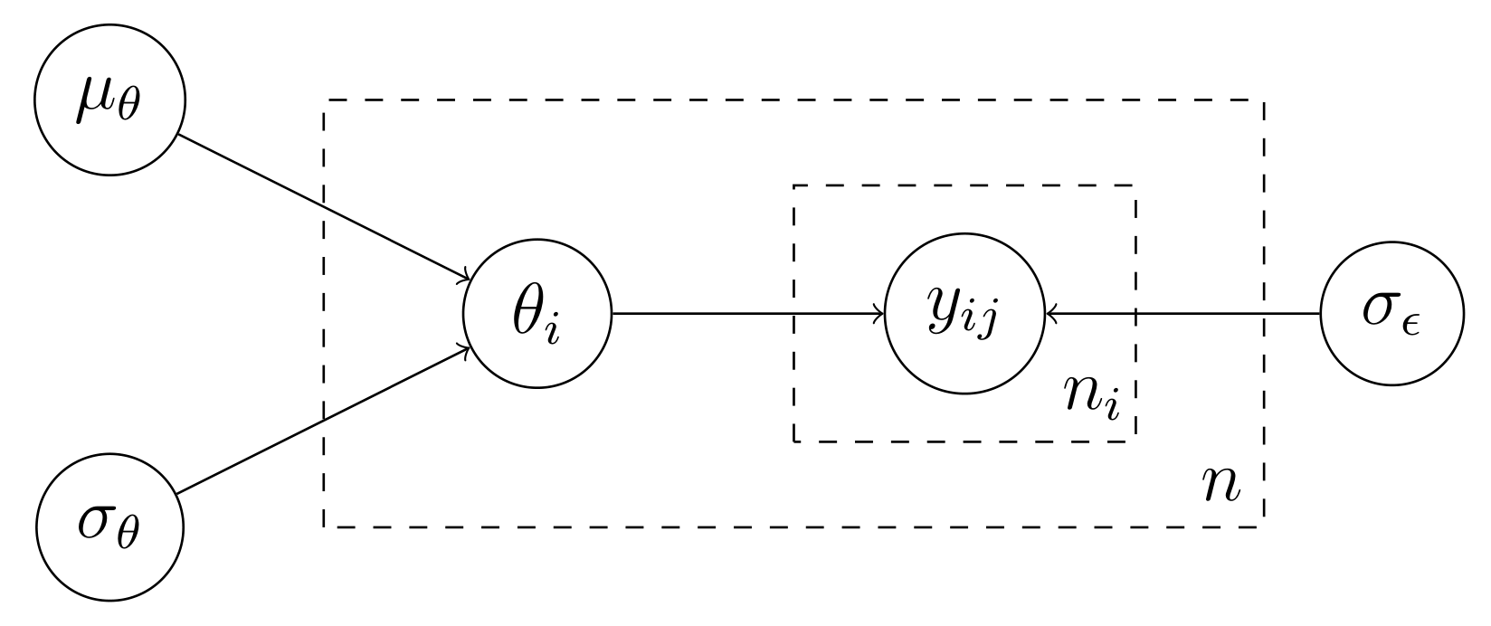
Thus, the model postulates that the outcome $Y_{ij}$ is generated by a two-step process. First, we draw the group $\theta_i \sim \text{Normal}(\mu_\theta, \sigma_\theta)$ and, then, we draw $Y_{ij} \sim \text{Normal}(\theta_i, \sigma_\epsilon)$. Now, suppose we observe a matrix of outcomes $\mathbf y$ that comes from this data-generating process, and we want to estimate its parameters via maximum likelihood. For the $i$th group, the likelihood contribution is given as
\[p(\mathbf y_i \,\vert\, \mu_\theta, \theta_i, \sigma_\theta, \sigma_\epsilon) = \prod_{j=1}^{n_i}p(y_{ij}\,\vert\, \theta_i,\mu_\theta, \sigma_\theta, \sigma_\epsilon)\]where $n_i$ is the number of individuals in group $i$ and where the joint density factors into a product as the $Y_{ij}$’s are independent given $\theta_i$ (see the DAG). So, the likelihood of the data can be formulated as
\[\begin{aligned} p(\mathbf y \,\vert\, \boldsymbol\theta, \mu_\theta, \sigma_\theta, \sigma_{\epsilon}) &= \prod_{i=1}^n \prod_{j=1}^{n_i} p(y_{ij}\,\vert\, \theta_i,\mu_\theta, \sigma_\theta, \sigma_{\epsilon}) \\ &= \prod_{i=1}^n \prod_{j=1}^{n_i}\text{Normal}(y_{ij} \,\vert\, \mu_\theta+\theta_i, \sigma_\epsilon) \\ &= \prod_{i=1}^n \prod_{j=1}^{n_i}\left(\frac{1}{\sqrt{2\pi}\sigma_\epsilon^2}\exp\left[-\frac{(y_{ij} - \theta_i - \mu_\theta)^2}{2\sigma_{\epsilon}^2}\right]\right). \end{aligned}\]The problem is that we cannot maximize this likelihood directly as $\theta_i$ appears in the last expression. We might treat the vector $\boldsymbol\theta$ as parameters to be estimated; but then, we would have to deal with the incidental parameter problem. Of course, for this special model, we might use the Least Squares Estimator to obtain unbiased estimates of $\boldsymbol\theta$. However, this will not work in the general case where the Least Squares Estimator is not a feasible choice, e.g., if this were a multilevel logit model.
So, what is usually done is to integrate the $\boldsymbol\theta$ out from the likelihood, which gives the marginal likelhood. Again, let us focus on the $i$th group. The contribution of the group to the marginal likelihood is
\[\begin{aligned} p(\mathbf y_i \,\vert\, \mu_\theta, \sigma_\theta, \sigma_{\epsilon}) &= \int p(\mathbf y_i, \theta_i \,\vert\, \mu_\theta, \sigma_\theta, \sigma_{\epsilon}) d\theta_i \\ &= \int p(\mathbf y_i \,\vert\, \mu_\theta, \theta_i,\sigma_\theta, \sigma_{\epsilon}) p(\theta_i\,\vert\, \mu_\theta, \sigma_\theta, \sigma_\epsilon)d\theta_i \\ &=\int \prod_{j=1}^{n_i}\text{Normal}(y_{ij} \,\vert\, \mu_\theta + \theta_i, \sigma_{\epsilon}) p(\theta_i\,\vert\, \mu_\theta, \sigma_\theta)d\theta_i \end{aligned}\]The marginal log-likelihood of the data, therefore, looks something like this:
\[\log p(\mathbf y\,\vert\, \mu_\theta,\sigma_\theta, \sigma_\epsilon) = \sum_{i=1}^n \log\left[\int \prod_{j=1}^{n_i}\text{Normal}(y_{ij} \,\vert\, \mu_\theta + \theta_i, \sigma_{\epsilon}) p(\theta_i\,\vert\, \mu_\theta, \sigma_\theta)d\theta_i\right].\]Now, this looks quite ugly. The important point, however, is that $\boldsymbol\theta$ is integrated out, so that the marginal log-likelihood will have no $\theta_i$ terms in it. Thus, if we could somehow evaluate that integral, we could maximize the marginal log-likelihood using conventional methods.
A second look at the last equation reveals that the integral is in fact an expectation over the distribution of $\theta_i$, i.e.,
\[\int \prod_{j=1}^{n_i}\text{Normal}(y_{ij} \,\vert\, \mu_\theta + \theta_i, \sigma_{\epsilon}) p(\theta_i\,\vert\, \mu_\theta, \sigma_\theta)d\theta_i = \text{E}_{\theta_i}\left[\prod_{j=1}^{n_i}\text{Normal}(y_{ij} \,\vert\, \mu_\theta + \theta_i, \sigma_{\epsilon})\right].\]This suggests that we can approximate the integral by
\[\text{E}_{\theta_i}\left[\prod_{j=1}^{n_i}\text{Normal}(y_{ij} \,\vert\, \mu_\theta + \theta_i, \sigma_{\epsilon})\right] \approx \frac{1}{S}\sum_{s=1}^S \left[\prod_{j=1}^{n_i}\text{Normal}\Big(y_{ij} \,\vert\, \mu_\theta + \theta_i^{(s)}, \sigma_{\epsilon}\Big)\right],\]where $\theta_i^{(s)}$ is the $s$th simulation draw from a $\text{Normal}( \mu_\theta,\sigma_\theta)$ distribution. By the (strong) Law of Large Numbers, the right hand side of the equation will converge (almost surely) to the desired expectation as $S\rightarrow \infty$. Thus, the simulated maginal log-likelihood is
\[\log p(\mathbf y\,\vert\, \mu_\theta,\sigma_\theta, \sigma_\epsilon)_{\text{Sim}} = \sum_{i=1}^n \log\left\{\frac{1}{S}\sum_{s=1}^S \left[\prod_{j=1}^{n_i}\text{Normal}\Big(y_{ij} \,\vert\, \mu_\theta + \theta_i^{(s)}, \sigma_{\epsilon}\Big)\right]\right\},\]which can be maximized with respect to $(\mu_\theta, \sigma_\theta, \sigma_\epsilon)$.
Okay. This looks ugly as well…But it turns out that writing a code for maximum simulated likelihood estimation (MSLE) is quite simple. But before going into coding it up, notice that the expression is quite general. The marginal distribution of $\theta_i$, $p(\theta_i \,\vert\, …)$, does not have to be the Normal distribution but might be any distribution from which we can sample.
Let us simulate some data with $\mu_\theta = 1.5, \sigma_\theta = 2, \sigma_\epsilon = 1$. We also set the number of groups to $n=50$ and the number of individuals within each group to $n_i = m = 10$ :
# set random seed

set.seed(321)

# parameters

mu.theta <- 1.5
sigma.theta <- 2
sigma.e <- 1

# group sizes

n <- 50
m <- 10
Next, we generate the data:
# random intercepts

n.dist <- rnorm(n, 0, sigma.theta)

# simulate data

y <- sapply(n.dist, function(w) mu.theta + w + rnorm(10,0,sigma.e))
The object y will have $n$ columns, for each group, and $m$ rows, for the $m$ individuals within each group. For any real implementation, it would be good to reshape the data into long-format in order to deal with missing values. But let us here just keep the data as they are.
One thing that was surprising to me at first, but which makes sense in hindsight, is that maximum simulated likelihood uses the same simulation draws for each iteration of the optimization procedure (see, for example, chapter 15 in Greene’s Econometric Analysis). That is, we first draw n.sim random numbers from $\text{Uniform}(0,1)$ for each group, and use the same draws to evaluate the expectation. To be more concrete, note that
where $\Phi$ is the standard Normal CDF. This method of generating random draws from a distribution is often called inverse transform sampling. Thus, if we let $u_i^{(s)}$ be the $s$th simulation draw from a Uniform distribution for group $i$, we can generate the $s$th draw of $\theta_i$ by calculating
\[\theta_i^{(s)} = \mu_\theta + \sigma_\theta \Phi^{-1}(u_i^{(s)}).\]Notice that $\theta_i^{(s)}$ will not be the same in each iteration as $\mu_\theta$ and $\sigma_\theta$ will be updated throughout of the optimization procedure. Yet, the underlying uniform draws will be kept constant. In fact, we don’t even need to calculate $\Phi^{-1}(u_i^{(s)})$ in each iteration; instead, we transform all the $u_i^{(s)}$ in advance, store them in an array, and extract the values whenever we need them.
So, let us first draw $3,000$ random numbers from $\text{Uniform}(0,1)$:
# number of draws for each group

n.sims <- 3000

# generate n times n.sims matrix to be used in optimization

sims <- matrix(runif(n * n.sims), ncol = n)

# generate corresponding Normal(0,1) draws

q.sims <- qnorm(sims)
Next, we code up the simulated likelihood function. There are two features in the code that might be worth noticing. First, we parameterize the likelihood in terms of $\log \sigma_\theta$ and $\log \sigma_\epsilon$, so that we can optimize the function in an unconstrained space. Second, to evaluate the product
\[\prod_{j=1}^m \text{Normal}(y_{ij}\,\vert\, \theta_i^{(s)}, \sigma_\epsilon)\]in the integrand, we exponentiate the sum the log of the densities, i.e.,
\[\exp\left\{\sum_{j=1}^m \log \Big[\text{Normal}(y_{ij}\,\vert\, \theta_i^{(s)}, \sigma_\epsilon)\Big]\right\}.\]This will be in general slower but will help to prevent underflow in the case the densities evaluate to small numbers.
sim.mlm <- function(pars, y, q.sims) {

    # parameters to be optimized

    mu.theta <- pars[1]
    lsigma.theta <- pars[2]
    lsigma.e <- pars[3]

    # calculate expected likelihood for ith group

    ll.i <- sapply(1:ncol(y), function(yi) {

        # generate draws of theta ~ Normal(mu.theta, sigma.theta)

        sim.theta <- mu.theta + exp(lsigma.theta) * q.sims[,yi]

        # for each draw of theta calculate the product over individuals

        mean(

            sapply(sim.theta, function(theta.i) {

                exp(sum(dnorm(y[,yi], theta.i, exp(lsigma.e), log = T)))

            })
        )
    })

    # return log-likelihood

    return(sum(log(ll.i)))

}

# bytecode compiling

sim.mlm <- compiler::cmpfun(sim.mlm)
Next, we generate initial values by linear regression and then maximize the simulated likelihood by a quasi-Newton routine. As the number of parameters is rather small and this is just a exercise, we don’t code up the gradient of the simulated log-likelihood, but rather approximate it numerically.
# run linear regression

inits.dat <- reshape2::melt(y); names(inits.dat) <-  c('id','i.id','y')
lm.fit <- lm(y ~ factor(i.id), data = inits.dat)

# initial values

inits <- numeric(3)
inits[1] <- coef(lm.fit)[1]
inits[2] <- log(sd(coef(lm.fit)[2:n]))
inits[3] <- log(summary(lm.fit)$sigma)

# maximize siulated likelihood using quasi-newton

opt.res = optim(par = inits,
                fn = sim.mlm,
                y = y,
                q.sims = q.sims,
                method = 'BFGS',
                control = list(trace = 1,
                               fnscale = -1,
                               REPORT = 5))

    initial  value 885.112118
    iter   5 value 802.450592
    iter  10 value 799.904624
    final  value 799.828796
    converged

# get estimates using lme4::lmer

library(lme4)
lmer.fit <- lmer(y ~ 1 | i.id, data= inits.dat, REML=F)

# compare results

res <- rbind(
    c(mu.theta, sigma.theta, sigma.e),
    c(opt.res$par[1], exp(opt.res$par[2]), exp(opt.res$par[3])),
    c(
        fixef(lmer.fit),
        sqrt(VarCorr(lmer.fit)$i.id[1,1]),
        summary(lmer.fit)$sigma
     )
)
rownames(res) <- c('True', 'Est.MSL','Est.lmer')
print(res)
## True 1.500000 2.000000 1.000000
## Est.MSL 1.688456 1.902594 1.002298
## Est.lmer 1.707071 1.868182 1.003145
Not bad (although it takes much longer than the lmer function)! A few considerations: we used $3,000$ simulation draws from the Uniform distribution in this example, but there are better ways to approximate the expectation in the likelihood. For example, using deterministic sequences of numbers in the interval $(0,1)$ designed to cover the interval uniformly, such as Halton draws, might reduce the number of draws needed and, thus, the computational burden. The randtoolbox::halton function might be used for this purpose. Also, in theory, the approximation to the expectation must converge faster than the marginal log-likelihood converges to its expectation in order for the maximum simulated likelihood estimator to be consistent. So the number $3,000$ used here will not always work.
Lastly, we used the fact that the Normal distribution belongs to the location-scale family of distributions. For other distributions, the trick of calculating
\[x = \text{location param.} + \text{scale param.} * Q(u),\]where $Q$ is the quantile function, will not work. This might slow down the optimization process considerably, especially for distributions for which $Q$ is expensive to calculate. For example, while the rate (or scale) parameter of the Gamma distribution has the same scaling property as the standard deviation of the Normal distribution, the the same does not hold for the shape parameter. In addition, the quantile function of a Gamma distribution has no closed-form, so that using inverse transform sampling is relatively inefficient compared to other methods used in generating Gamma variates (a comparison between qgamma(u), where u = runif(1), and rgamma(1) suggests that the former takes about 20 times more computational time). This can become a major burden for applying maximum simulated likelihood estimation. For example, imagine using the inverse transform sampling to integrate out a parameter that follows a Dirichlet distribution, which, in turn, is simulated using a series of Gamma variates. It might not be worth the time…