Jacobian Adjustments in the Metropolis-Hastings Algorithm
DISCLAIMER: This is a blog post from my graduate school years. The blog is no longer maintained and the material might include typos and errors.
Suppose we want to sample from the distribution of a positive random variable $X$ with a random walk Metropolis-Hastings algorithm. There is nothing wrong with using a proposal distribution that might result in negative proposals in this situation. The negative proposals are simply rejected and the sampler will continue to sample from the correct target distribution. A shortcoming of this approach, however, is that, sometimes, too many of the proposals will be rejected, rendering the sampler inefficient. Therefore, it is often sensible to specify a proposal that has to be positive as well, such as the Gamma or the Pareto distribution, or to transform the variable into an unconstrained space and use Normally distributed proposals on the transformed space. It is the latter with which I am planning to deal in this post.
The following example might illustrate the point. Say, we want to sample from a $\text{Gamma(3,1)}$ density (where we use the shape-rate parameterization) by using Normally distributed proposals with variance $\delta^2$, i.e., $x^\ast \sim \text{Normal}(x, \delta)$, where $x^\ast$ is the proposed value and $x$ is the current value at each iteration. The acceptance ratio is then
\[r = \frac{\text{Gamma}(x^\ast\, \vert \, 3,1) \text{Normal}(x\, \vert \, x^\ast, \delta)}{\text{Gamma}(x \, \vert \, 3,1)\text{Normal}(x^\ast\, \vert \, x, \delta)} = \frac{\text{Gamma}(x^\ast\, \vert \, 3,1) }{\text{Gamma}(x \, \vert \, 3,1)}\]since the Normal distribution is symmetric—i.e., $\text{Normal}(x\, \vert \, x^\ast, \delta) = \text{Normal}(x^\ast\, \vert \, x, \delta)$. We accept the proposal with probability
\[\rho = \min\big\{1, r\big\}.\]So, the Metropolis-Hastings algorithm might be coded up as follows. Notice we calculate the acceptace ratio on the log-scale for numerical stability.
# draw from proposal distribution

proposal = function(x) { rnorm(1, x, delta) }

# log-acceptance ratio

log_ratio = function(xstar, x) {

    dgamma(xstar, 3, 1, log = T) - dgamma(x, 3, 1, log = T)

}

# define MH-sampler

SampleMH = function(
    x,             # initial value

    proposal.fun,  # proposal function

    log.accept,    # log-acceptance ratio

    n.sims) {      # number of samples to take


    # emprty container

    samps = numeric(n.sims)

    # start sampling

    for (n in 1:n.sims) {

        # draw proposal

        xstar = proposal.fun(x)

        # accept if rho > runif(1)

        if (log.accept(xstar, x) >= log(runif(1)))
            x = xstar

        samps[n] = x

    }

    return(samps)
}


# parameters & initial value

set.seed(123)
n.sims = 5e5
delta = 1
x = 2

samps = SampleMH(
        x = x,
        proposal.fun = proposal,
        log.accept = log_ratio,
        n.sims = n.sims
    )
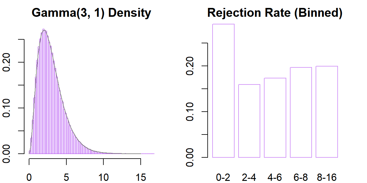
The results show that the algorithm successfully approximates the target distribution:
par(mfrow = c(1, 2), mar = rep(2, 4))

# grid & colors

gd = seq(0, 15, .1)
purple.5 = scales::alpha("purple", .5)

# histogram

hist(samps, freq = F, xlab = "", ylab = "", breaks = 100,
     border = purple.5, main = "Gamma(3, 1) Density")
lines(gd, dgamma(gd, 3, 1), col = "grey50")

# rejections

ints = c(seq(0, 8, 2), 16)
reject = cbind(
    as.numeric(diff(samps) == 0),
    findInterval(samps[-1], ints, all.inside = T)
)
barplot(
    tapply(reject[, 1],
           reject[, 2],
           mean),
    border = purple.5,
    col = "white",
    names.arg = zoo::rollapplyr(
        ints, 2, FUN = paste0, collapse = "-", by = 1
    ),
    main = "Rejection Rate (Binned)")
At the same time, however, we see that a lot of propsals near zero are rejected. This is expected: if the current state of the sampler is near zero, the next proposal will have a high probability of being negative, which leads to an automatic rejections.
So, one might wonder why not using a proposal distribution that is strictly positive? One way to do so is to sample on the log-scale. That is, we keep the Normally distributed proposal distribution but sample
\[\log(x^\ast) \sim \text{Normal}(\log(x),\delta)\]and then use $x^\ast = \exp(\log(x^\ast))$ as our proposed value. This ensures that all proposals will be strictly positive, preventing the high rate rejections near $x^\ast=0$. Also, as before, $\text{Normal}(\log(x^\ast)\, \vert \, \log(x), \delta) = \text{Normal}(\log(x)\, \vert \, \log(x^\ast),\delta)$, so can use the exact same acceptance ratio.
# draw from proposal distribution

# xstar = exp(ystar)

proposal = function(x) { exp(rnorm(1, log(x), delta)) }

# run sampler

samps = SampleMH(
        x = x,
        proposal.fun = proposal,
        log.accept = log_ratio,
        n.sims = n.sims
    )

# histogram

par(mfrow = c(1,1))
hist(samps, freq = F, xlab = "", ylab = "", breaks = 100,
     border = purple.5, main = "Gamma(3, 1) Density")
lines(gd, dgamma(gd, 3, 1), col = "grey50")
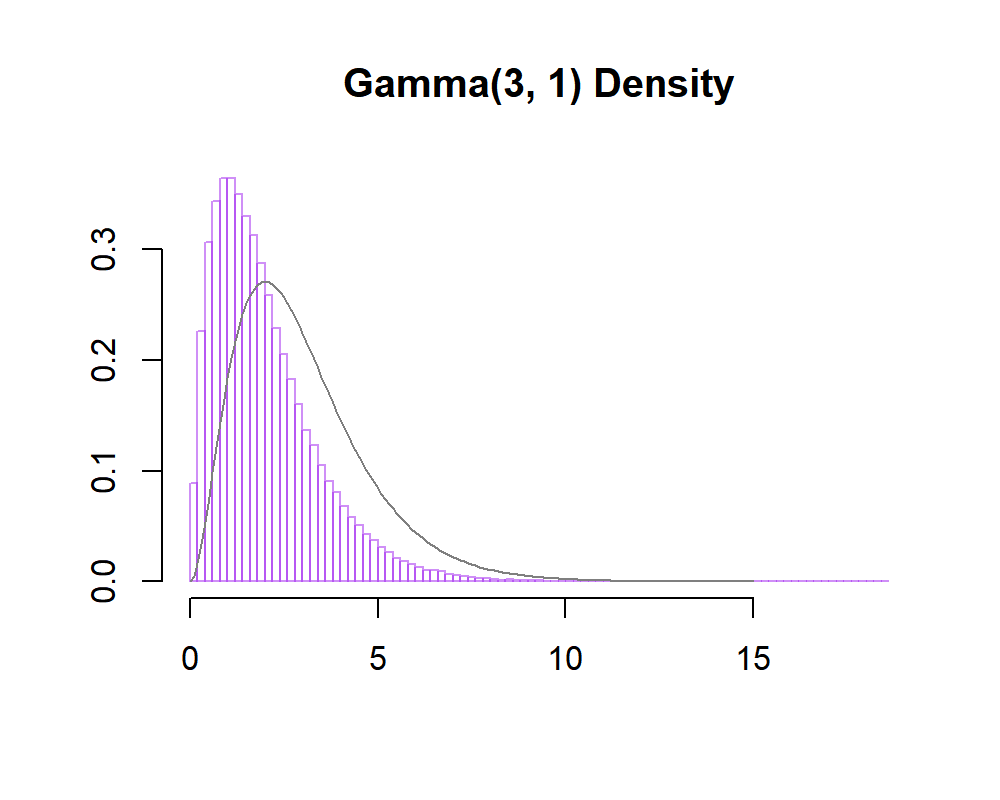
Yet, as the figure above shows, once we switch to the log-scale the sampler fails to sample from the traget distribution. The reason for its failure lies the fact that we have changed variables and forgot to adjust for this . In order to see where the algorithm went wrong, consider again the expression
\[\log(x^\ast) \sim \text{Normal}(\log(x), \delta).\]This is a probabilistic statement about $\log(x^\ast)$ and not $x^\ast$. On the other hand, in calculating the acceptance ratio, $\rho$, we need to account for the probability that $x^\ast$ is proposed from state $x$, and vice versa, not the probability of $\log(x^\ast)$ and $\log(x)$.
To adjust for the change of variables, we can rely on a simple theorem about the distribution of functions of random variables. The general formula can be found in most introductory statistics textbooks and is based on a standard result in calculus. The version below is from Mood et al.’s introductory book with minor changes in notation:
Theorem (Change of Variables, Unidimensional, Continuous)
Suppose $W$ is a continuous random variable with probability density function $f_W$. Set $\mathcal W = \{w: f_W(w) > 0\}$. Assume that
- $g: \mathcal W \rightarrow \mathcal V$ defines a one-to-one transformation of $\mathcal W$ onto $\mathcal V$.
- The derivative of $w = g^{-1}(v)$ with respect to $v$ is continuous and nonzero for $v\in \mathcal V$, where $g^{-1}(v)$ is the inverse function of $g(w)$; that is, $g^{-1} (v)$ is that $w$ for which $g(w) = v$.
Then $V = g(W)$ is a continuous random variable with density
\[f_V(v) = \left\vert \frac{\,\text{d}}{\,\text{d} v}g^{-1}(v)\right\vert f_W(g^{-1}(v)) \mathbb I_{\mathcal V} (v).\]The term that appears in the absolute value function is called the Jacobian of the transformation. Intuitively, the Jacobian of a function $f$ evaluated at the point $x$ can be understood as the amount to which a function stretches or contracts volumes near the point $x$. This also gives some intuition about why it appears whenever we want to change variables, either in the univariate context or the multivariate context.
Now, back to the problem. We know that the proposal $\log(x^\ast)$ is Normally distributed with mean $\log(x)$ and standard deviation $\delta$, but we are interested in the distribution of $x^\ast$. To align the notation with that of the theorem, let
\[\log(x^\ast) = w\quad \text{ and }\quad x^\ast = v.\]The mapping that transforms $w$ to $v$ is the exponential function and its inverse is the logarithm. Thus, $g(w) = \exp(w)$ and $g^{-1}(v) = \log(v)$. The exponential function, indeed, defines a one-to-one transformation of $\mathcal W = \mathbb R$ onto $\mathcal V = \mathbb R_+$; and $g^{-1}$ is continuously differentiable with respect to $v$ and is non-zero on $\mathbb R_+$. So, all requirements to apply the change of variable formula are satisfied.
Applying the formua, we obtain
\[\begin{aligned} f_{V}(v) &= \left\vert\frac{\,\text{d}}{\,\text{d} v} g^{-1}(v)\right\vert f_{W}(g^{-1}(v)) \\ &= \left\vert\frac{\,\text{d}}{\,\text{d} v} \log(v)\right\vert f_{W}(\log(v)) \\ &= \left\vert\frac{1}{v}\right\vert\text{Normal}\Big(\log(v)\,\Big\vert\, \log(x), \delta\Big), \end{aligned}\]for $v > 0$. So,
\[f_{X^\ast}(x^\ast) = \left\vert\frac{1}{x^\ast}\right\vert\text{Normal}\Big(\log(x^\ast)\,\Big\vert\, \log(x), \delta\Big)\]and we see immediatly that the Jacobian is the missing piece we’ve left out.
Lastly, to incorporate the Jacobian, we note that the acceptance ratio is calculated on the log-scale. So, we have to add (not multiply)
\[\log\left\vert\frac{\,\text{d}}{\,\text{d} x} \log(x)\right\vert = \log \left\vert \frac{1}{x}\right\vert = -\log(x)\]and $-\log(x^\ast)$, respectively, from the numerator and denominator in the acceptance ratio.
So let’s run the sampler again:
# draw from proposal distribution (same as before)

proposal = function(x) { exp(rnorm(1, log(x), delta)) }

# Jacobian adj.

log_jacobian = function(x) { -log(x) }

# new log-acceptance ratio (with Jacobian adj.)

log_ratio_adj = function(xstar, x) {

    dgamma(xstar, 3, 1, log = T) +
        (dnorm(log(x), log(xstar), delta, log = T) + log_jacobian(x)) -
        dgamma(x, 3, 1, log = T) -
        (dnorm(log(xstar), log(x), delta, log = T) + log_jacobian(xstar))

}

# run sampler with Jacobian adj.

samps = SampleMH(
        x = x,
        proposal.fun = proposal,
        log.accept = log_ratio_adj,
        n.sims = n.sims
    )
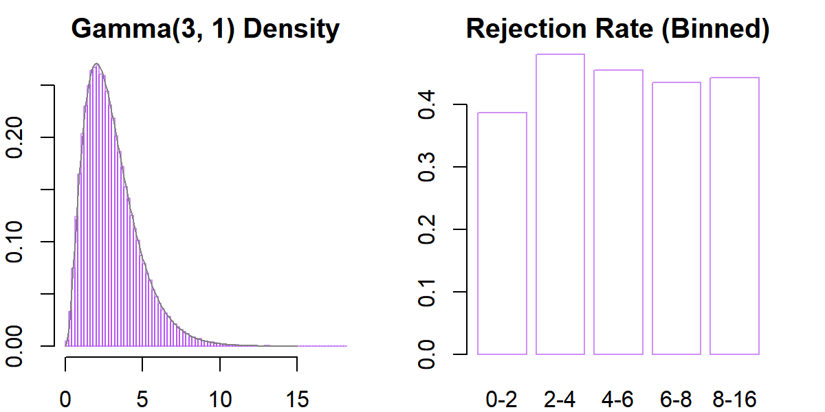
The results look as follows:
# histogram

par(mfrow = c(1,2), mar = rep(2,4))
hist(samps, freq = F, xlab = "", ylab = "", breaks = 100,
     border = purple.5, main = "Gamma(3, 1) Density")
lines(gd, dgamma(gd, 3, 1), col = "grey50")

# rejections

ints = c(seq(0, 8, 2), 16)
reject = cbind(
    as.numeric(diff(samps) == 0),
    findInterval(samps[-1], ints, all.inside = T)
)
barplot(
    tapply(reject[, 1],
           reject[, 2],
           mean),
    border = purple.5,
    col = "white",
    names.arg = zoo::rollapplyr(
        ints, 2, FUN = paste0, collapse = "-", by = 1
    ),
    main = "Rejection Rate (Binned)")
Voila! Looks good!