Entropy
DISCLAIMER: This is a blog post from my graduate school years. The blog is no longer maintained and the material might include typos and errors.
Most students, at least in sociology, think of “uncertainty” in statistics in relation to “variances” or “standard deviations.” This is only natural: the “standard error” is the standard deviation of the sampling distribution of an estimator under a specified null hypothesis; the “uncertainty” in fitted models is often summarized by the variance-covariance matrix, and so on.
Yet, to be exact, the variance is just the average squared distance from the mean of a distribution, not a measure of “uncertainty” in general, especially if we mean by uncertainty our lack of knowledge regarding an outcome. Further, our intuitions regarding the variance of a distribution often fails, when the distribution is not symmetric. But then, what other measure should we use to quantify “uncertainty”? What properties should a measure of “lack of knowledge” satisfy? It is out of these questions that the measure of “entropy” emerged in information theory.
But what is this thing called entropy? For someone, like me, not familiar with information theory (or statistical mechanics), the term entropy has some mystical qualities and, historically, that was one of the reasons why Shannon named his measure in this way. According to Myron Tribus, Claude Shannon said:
My greatest concern was what to call it. I thought of calling it 'information,' but the word was overly used, so I decided to call it 'uncertainty.' When I discussed it with John von Neumann, he had a better idea. Von Neumann told me, 'You should call it entropy, for two reasons. In the first place your uncertainty function has been used in statistical mechanics under that name, so it already has a name. In the second place, and more important, no one knows what entropy really is, so in a debate you will always have the advantage.'
Anyways, by following how Shannon came up with this measure, we might gain some insights into what entropy means.
Derivation of Shannon's Information Entropy
Let $ \Pi_n=\{p_1,…,p_n\} $ be a probability distribution. The information entropy, or simply entropy, of this distribution is given as
\[H(\Pi_n) = H_n = -\sum_{i=1}^n p_i \log p_i,\]In 1948, Shannon published an influential article in the Bell System Technical Journal under the name “A Mathematical Theory of Communication.” There, he argued that a measure of “unceratinty” regarding the outcome drawn from a distribution $ \Pi_n $ should satisfy the following three conditions:
- $ H $ is continuous in $ p_i $.
- If $ p_i = 1/n $, for all $ i $, then $ H $ increases monotonically in $ n $.
- “If a choice be broken down into two successive choices, the original $ H $ should be the weighted sum of the individual values of $ H $.’’ (p.393.)
Condition (1) simply states that “small” difference in the probabilities should lead to “small” changes in the uncertainty measure; without this condition an $ \epsilon $ change in $ p_i $ can lead to an infinite change in $ H $, which is undesirable. Condition (2) makes also intuitive sense: it states that when all outcomes are equally likely, our uncertainty measure should be greater for distributions with many outcomes. Condition (3) might need a little bit more elaboration. Consider drawing a ball from a jar of 6 balls out of which 3 are red, 2 are blue, and 1 is green. The probability of drawing a red, blue, or green ball is given, in order, by the probabilities $ \{1/2,1/3,1/6\} $. Yet, we might arrive at the same probability distribution in another way. Namely, we might first choose whether to draw a red ball or not, with probability 1/2 for each outcome, and if we have decided not to choose a red ball, we draw a blue or green ball with probability 2/3 and 1/3, respectively. Condition (3) states that we should be able to recover the entropy of the probability distribution of drawing a ball from the jar at once as the weighted sum of the two-step method. That is,
\[H(1/2,1/3,1/6) = H(1/2,1/2) + \frac{1}{2}H(2/3,1/3).\]The important point here is that the left hand-side can be expressed as a weighted sum, not a product or more complicated function. In this particular case, the weight on the second term is 1/2 as case occurs only half of the time.
More formally, if we have a compound experiment, $ AB $, consisting of two stages, first $ A $ with $ m $ possible outcomes $ A_1,…,A_m $ occurring with probabilities $ p_1,…,p_m $, and then $ B $, our uncertainty measure for the the compound experiment, $ H(AB) $, should satisfy the relation
\[H(AB) = H(A) + \sum_{k=1}^m p_k H(B\,\vert\, A_k).\]It turns out that the only measure that satisfies the three conditions is the entropy $ H $ as it was defined above.
The derivation of the result is quite straightforward. Let $ A(\cdot) $ be a measure that satisfies (1) to (3). Define $ A(k) = \{1/n_1,1/n_2,…,1/n_k\}$ with $n_i = n_j$ for all $i,j\le k$. That is $A(k)$ is the value of the measure $A$ for a random variable with $k$ equiprobable outcomes. Consider $A(s m)$. By property (3), we can break down the choice from $sm$ equiprobable outcomes into a choice of $m$ equiprobable sets of outcomes, each of which will have again $s$ outcomes with equal probability. Thus,
\[A(sm) = A(m) + \sum_{j=m}^s p_j A(s) = A(m) + \sum_{j=1}^m \frac{1}{m} A(s) = A(m) + A(s).\]That the measure of an input in the form of a product is equal to the sum of the measures of the terms in the product is revealing. Indeed, we see that this property is satisfied by the logarithm and that \(A(m) = K\log m\) for an arbitrary constant $K$, which has to be positive to satisfy axiom (2). This shows that a measure $ H $ of “uncertainty” that satisfies condition (2) and (3) must have a form of $ H_n = K\log n $ for a distribution with $ n $ equiprobable outcomes.
Now, consider a set of $ n $ possible events with equal probability of occurring that lead to $ m $ distinguishable outcomes. We might group the events that lead to the same outcome $1\le i \le m$ together and assign probabilities $ p_i = n_i/n $ to each of them, where $ n_i $ is an integer that represents the number of events leading to outcome $ i $. By property (3), we have
\[A\left(\sum_i n_i\right) = A(p_1,...,p_n) + \sum_{i} p_i A(n_i)\]But as $ A(\sum_i n_i) = K\log (\sum_i n_i) $ and $ A(n_i) = K \log n_i $, this can be written as
\[K \log \left(\sum_i n_i\right) = A(p_1,...,p_n) + K\sum_{i} p_i \log n_i.\]It follows that
\[\begin{aligned} A(p_1,...,p_n) &= K\left[\log \left(\sum_i n_i\right) - \sum_i p_i \log n_i\right] \\ &= K\left[\sum_i p_i \log \left(\sum_i n_i\right) - \sum_i p_i \log n_i\right] \\ &= K\left[ \sum_i p_i \log \left(\frac{\sum_i n_i}{n_i}\right)\right] \\ &= - K \sum_i p_i \log p_i \end{aligned}\]as desired. Lastly, if the $ p_i $’s cannot be expressed as rationals, condition (1) ensures that that the same equation must still hold for irrationals. This completes the derivation.
Alternative Motivation
An alternative derivation of the entropy measure can be motivated by following thought experiment. Suppose we want to draw $ n $ numbers with replacement from the set $ \{1,2,…,m\} $. We want that each number has the same probability of being drawn, $ 1/m $, and that each draw is independent. In short, we want the most uniform random experiment possible. Suppose we run this experiment for a large number of times. Each run of the experiment will result in a different distribution of outcomes: for some runs, we will draw the number 1 $ n $ times; for other runs we obtain the number $ 1,2,…,m $ an equal number of times, and so on. Now, given this setup, we ask “what is the most likely distribution to arise?”. From a Frequentists’ view point, this question is equivalent to asking “if we would run these experiments an infinite number of times, what is the distribution with highest probability (i.e, relative frequency of occurring)?”
The key insight to answer this question is the realization that there is a huge variation in the number of ways a certain collection of numbers can be drawn. For example, there is exactly one way to draw “1” $ n $ times; but there are $ n!/m!(n-m)! $ ways to draw a “2” $ m < n $ times and a “3” $ n-m $ times. In general, the number of ways in which a sample with $ n_1 $ ones, $ n_2 $ twos, ….,$ n_m $ “m”s can be drawn is given by the multinomial coefficient
\[W = \frac{n!}{n_1!n_2!\cdots n_m!} = \binom{n}{n_1,n_2,...,n_m}\]and the probability of observing such a collection of draws is thus
\[\Pr[n_1,...,n_m] = \binom{n}{n_1,...,n_m} \prod_{i=1}^m \left(\frac{1}{m}\right)^{n_i}\propto W,\]as the product $ \prod_i m^{-n_i} = m^{-n} $ is a constant. Thus, the distribution that maximizes $ W $ will be the distribution that we will observe most frequently.
Now, consider
\[\frac{1}{n}\log W = \frac{1}{n}\left(\log n! - \sum_{i=1}^n \log n_i!\right)\]Approximating $ n! $ by Stirling’s formula $ \log n! = n \log n -n + O(\log n) $, we obtain
\[\frac{1}{n}\log W \approx \frac{1}{n}\left( n \log n - n - \sum_{i=1}^m (n_i\log n_i - n_i)\right)= \frac{1}{n}\left( n \log n - \sum_{i=1}^m n_i\log n_i \right).\]Lastly, let $ p_i = n_i/n $ be the relative frequency of drawing number $ i $ and substitute this expression to get
\[\begin{aligned} \frac{1}{n}\log W &\approx \frac{1}{n}\left(n \log n - \sum_{i=1}^m (n p_i) \log (n p_i)\right) \\ &=\frac{1}{n}\left(n\log n - \left[n\sum_{i=1}^m p_i \log p_i + n\sum_{i=1}^m p_i\log n\right]\right)\\ &= - \sum_{i=1}^m p_i \log p_i \end{aligned}\]which is the formula of the information entropy. As maximizing $ W $ is equivalent to maximizing $ n^{-1}\log W $, it follows that the probability distribution we are seeking is the distribution that has the maximum entropy. Thus, the maximum entropy distribution is the most probable distribution in that it has the largest number of possible ways to be realized given that we draw the numbers as random as possible.
An Illustration
Consider $ m=4 $ possible outcomes, $ M=\{1,2,3,4\} $. For each run of our experiment, we use $ n=20 $ trials of drawing a random number (with replacement) from the set $ M $.
n= 20
k= 4
As mentioned above, there is only one way in which we might draw $ n $ times a $ 1 $. The uniform distribution, with 5 draws of each number, has on the other hand
exp(lfactorial(n) - k*lfactorial(n/k))[1] 11732745024
ways to be drawn (this is why we used $ n=20 $ and not a larger number). Comparing this to the number of possible realizations of a distribution which deviates from the maximum entropy distribution by the slightest possible degree, we get
exp(
  lfactorial(n) -
  lfactorial(n/k - 1) -
  (k - 2) * lfactorial(n/k) -
  lfactorial(n/k + 1)
)
[1] 9777287520
which is a difference of 1,955,457,504. In other words, the (discrete) uniform distribution has a much higher probability to arise.
We might also directly simulate the experiment. First, we load some packages.
library('data.table')
library('dplyr')
library('ggplot2')
Now, the number of different types of samples that might be obtained from drawing 20 numbers from a set of 4 is
choose(n + k - 1, k - 1)[1] 1771
by the stars-and-bars type of argument. That is, we might think of the number of ways to put $ n $ balls into $ k $ urns as a problem of deciding the position of $ k-1 $ bars between $ n $ stars. This will partition the $ n $ stars (balls) into $ k $ bins (urns). As there are $ n+k-1 $ places to put the bars, and the positions of the stars are perfectly determined (given that they are indistinguishable) once we know the positions of the bars, the total number of arrangements is given as $ \binom{n+k-1}{n} $. Note that this is also the number of all possible combinations of $ k $ positive integers that sum to $ n $.
Back to our experiment. Let us draw a large number of experimental runs, here 5 million:
# set seed

set.seed(123)

# draw balls from 1,...,k with equal probability

z <- rmultinom(5000000, n, prob = rep(1, k)) %>%
  t %>%
  data.table

  # count the number of each drawn combination

dat <- z[, .N, by = eval(paste0('V', 1:k))]
Next, we calculate the entropy of each realized distribution and plot the results:
# calculate entropy

dat[, ent := apply(
    dat[, paste0('V', 1:k), with = F],
    1,
    function (w) {
        p <- w/n
        -sum(ifelse(p == 0, 0, p * log(p)))
    })
]

# plot results

ggplot(dat, aes(x = ent, y = N)) +
  geom_point(col = viridis::viridis(1),
             alpha = .4,
             size = .9) +
  geom_vline(xintercept = log(k),
             linetype = 2) +
  scale_y_continuous(
    breaks=c(
      seq(1, dat[!which.max(N), max(N)], length.out = 5),
      dat[, max(N)]
    )
  ) +
  labs(x = 'Entropy', y = 'No. of Occurences') +
  theme_bw()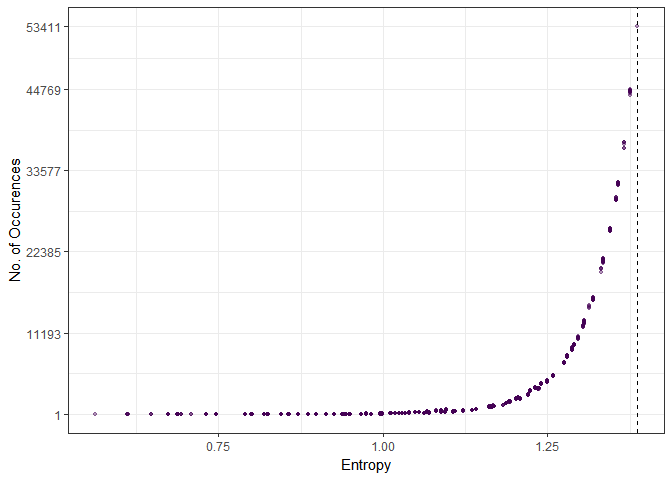
The dashed line shows the maximum entropy value, which corresponds to the uniform distribution with 53,411 occurences. The top 13 distributions that were drawn are
dat[order(-N)][1:13] V1 V2 V3 V4 N ent
1: 5 5 5 5 53411 1.386294
2: 5 4 5 6 44769 1.376227
3: 4 6 5 5 44661 1.376227
4: 5 5 6 4 44629 1.376227
5: 5 4 6 5 44562 1.376227
6: 5 5 4 6 44536 1.376227
7: 4 5 6 5 44498 1.376227
8: 5 6 5 4 44495 1.376227
9: 6 5 4 5 44431 1.376227
10: 5 6 4 5 44400 1.376227
11: 4 5 5 6 44377 1.376227
12: 6 5 5 4 44150 1.376227
13: 6 4 5 5 43979 1.376227
Note that these are 1) the maximum entropy distribution and 2) the $ 2\binom{k}{2}=12 $ distributions that diverge by the slightest possible degree from the uniform distribution. On the other hand, if we look at the least often occuring distributions, we find that they have substantially lower entropy, meaning that the distributions are much more “concentrated” around specific values.
dat[order(N)][1:10] V1 V2 V3 V4 N ent
1: 15 3 2 0 1 0.7305881
2: 15 1 1 3 1 0.7999028
3: 15 4 1 0 1 0.6874358
4: 11 0 9 0 1 0.6881388
5: 0 2 14 4 1 0.8018186
6: 11 9 0 0 1 0.6881388
7: 0 11 9 0 1 0.6881388
8: 6 0 13 1 1 0.7909874
9: 1 3 1 15 1 0.7999028
10: 4 1 15 0 1 0.6874358
Note also that none of the distributions with entropy zero (namely those where the same number is drawn $ n $ times) have occurred.
cols <- paste0('V',1:k)
dat[dat[,Reduce('+',lapply(.SD,'==',n)), .SDcols=cols]]
Empty data.table (0 rows) of 6 cols: V1,V2,V3,V4,N,ent
In fact, we can go one step further. Suppose that we want our outcomes of the experiment to satisfy a set of constraints. In other words, we are seeking the distribution that has the highest probability of realizing under an experiment that is uniformly random as possible given a set of constraints. In intuitive terms, this means that except for the specified constraints, we assume that we have “no knowledge” of the distribution. Say we want the distribution to satisfy the condition that the number {1} is drawn at least 7 times.
dat2 <- dat[V1>=7]
ggplot(dat2, aes(x=ent, y=N)) +
  geom_point(col=viridis::viridis(1),
             alpha=.4,
             size=.9) +
  geom_vline(xintercept=log(k),
             linetype=2) +
  labs(x='Entropy', y='No. of Occurences') +
  theme_bw()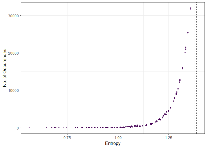
Again, we see the same result: higher entropy, more occurences. Checking the distributions that were observed the most, we see immediately that the most frequently occuring distributions are those that spread the “data” as uniformly across the outcomes as possible.
dat2[order(-N)][1:10]This becomes more evident if we enforce an additional constraint.
dat3 <- dat[V1>=7 & V2>=7]
dat3[order(-N)][1:10]
V1 V2 V3 V4 N ent
1: 7 7 3 3 12198 1.304011
2: 7 7 2 4 9197 1.287022
3: 7 7 4 2 8968 1.287022
4: 7 8 3 2 4587 1.248781
5: 8 7 2 3 4463 1.248781
6: 7 8 2 3 4459 1.248781
7: 8 7 3 2 4406 1.248781
8: 7 7 5 1 3618 1.231236
9: 7 7 1 5 3614 1.231236
10: 7 8 4 1 2303 1.205628
Maximum Entropy Distributions
Maximum entropy distributions offer a convenient choice in deciding among priors for parameters according to the principle of insufficient reason. In other words, given that we have no knowledge about the likelihood of an outcome occurring, we should assign each outcome an equal probability. For example, suppose you have a parameter, $ \theta $, that is defined on the real line for which you have to choose a prior. We want the prior to satisfy one constraint, namely, that its variance is finite, i.e. $ \sigma^2 < \infty $, but otherwise we have no other prior beliefs regarding it. In terms of entropy, we are seeking the distribution that maximizes the entropy over all distributions defined over $ \mathbb R $ with finite variance $ \sigma^2 $. It turns out that the unique distribution satisfying these conditions is the Normal distribution. This result gives the Normal distribution another special place in statistics, justifying its wide use aside of the Central Limit Theorem.
To show that this is true, we first derive the entropy of the Normal distribution with variance $ \sigma^2 $. We define the entropy for a probability density function, $ p $, defined over the interval $ I $ as
\[H(p) = -\int_I p(x) \log p(x) \, dx\]where we set $ 0\log 0 = 0 $ as $ \lim_{z\rightarrow 0^+}z\log z=0 $.
Let $ \phi(z) $ denote the standard Normal pdf and let $ z= (x-\mu)/\sigma $. Then the entropy of a Normal distribution with mean $ \mu $ and variance $ \sigma^2 $ is
\[\begin{aligned} H(\phi) &= - \int_{\mathbb R} \frac{1}{\sigma}\phi\left(\frac{x-\mu}{\sigma}\right) \log\left[\frac{1}{\sigma} \phi\left(\frac{x-\mu}{\sigma}\right)\right] dx \\ &=- \int_{\mathbb R} \phi(z)\left[-\log\sigma +\log\phi(z)\right] dz \\ &= \log\sigma - \int_{\mathbb R}\left(-\frac{1}{2}\log(2\pi) - \frac{z^2}{2}\right)dz \\ &= \log\sigma +\frac{1}{2}\log(2\pi) + \frac{1}{2} \\ &= \frac{1}{2}[\log(2\pi \sigma^2) + 1] \end{aligned}\]as $ \int_{\mathbb R}\phi(z)dz = \int_{\mathbb R}z^2\phi(z)dz=1 $. Note that the mean of the distribution does not enter the expression, implying that all Normal distributions with the same variance have the same entropy.
By the Gibbs Inequality, we have that for two continuous density functions $ p\ge 0 $ and $ q>0 $ on an interval $ I\subset \mathbb R $,
\[-\int_I p(x)\log p(x) dx \le - \int_I p(x) \log q(x) dx\]if both integrals exists, and where the inequality holds as an equality if and only if $ p=q $ almost everywhere on $ I $. A trivial observation that follows from the Gibbs inequality, but which we will use below, is the following: If we have $ -\int_I p(x)\log q(x) dx = H(q) $, then $ H(p) \le H(q) $ on $ I $ with equality if and only if $ p=q $ almost everywhere on $ I $ (Just equate the left-hand side of the Gibbs inequality with $ H(p) $ and observe that the right-hand side is $ H(q) $).
Now, let $ \nu $ be an arbitrary continuous density function defined on $ \mathbb R $ with finite variance $ \sigma^2 $. Let $ \mu $ be it’s mean, which exists since the variance is finite. Let $ \phi $ be a Normal distribution with the same mean $ \mu $ and the same variance $ \sigma^2 $. Then, we have
\[\begin{aligned} - \int_{\mathbb R}\nu(x) \log \phi(x) dx &= -\int_{\mathbb R} \nu(x) \left[-\frac{1}{2}\log(2\pi\sigma^2) - \frac{1}{2\sigma^2} (x-\mu)^2 \right]dx \\ &=\frac{1}{2}\log(2\pi\sigma^2) + \frac{1}{2\sigma^2}\int_{\mathbb R}(x-\mu)^2\nu(x) dx \\ &= \frac{1}{2} \left[\log(2\pi\sigma^2) + 1\right] \\ &= H(\phi). \end{aligned}\]Therefore, $ H(\nu) \le H(\phi) $ on $ \mathbb R $, showing that the Normal distribution is the maximum distribution on $ \mathbb R $ with finite variance.
What about other distributions? Suppose we want to find the maximum entropy distribution on $ \mathbb R_+ $ with finite mean $ \lambda $. This time, let us use a different approach and maximize the entropy directly (recall that we started the discussion of the Normal with the prior knowledge that the Normal is the distribution we are looking for. This enabled us to use $ \phi $ in the position of $ q $ in the Gibbs inequality. If we had not known the results in advance, we would be lost.)
We start with three constraints: 1) the distribution is defined on the positive real line, 2) the distribution has to integrate to one, and 3) the mean is finite and equal to $ \lambda $. Thus, we set
\[\begin{aligned} G(\lambda, \mu_1,\mu_2) &= -\int p(x) \log p(x) dx + \mu_1 \left(\int p(x) dx - 1\right) + \mu_2 \left(\int x p(x) dx - \lambda\right) \\ &=\int\Big[-p(x)\log p(x) + \mu_1 p(x) + \mu_2 xp(x)\Big] dx - \mu_1 - \mu_2 \lambda \\ &=\int \mathcal L(x, p(x), \mu_1,\mu_2) dx - \mu_1 - \mu_2\lambda \end{aligned}\]where integration over $ [0,\infty) $ is understood, $ \mu_1,\mu_2 $ are the Lagrangian multipliers, and $ \mathcal L(x,p,\mu_1,\mu_2) = -p \log p + \mu_1p + \mu_2 xp $. At a maximum, the first variation of the functional $ \mathcal L $ with respect to $ p $ has to satisfy
\[\frac{\delta \mathcal L}{\delta p} = -\log p -1 + \mu_1 + \mu_2 x = 0\]so that we have
\[p(x) = \exp(\mu_1 + \mu_2 x -1)\]for $ x\ge 0 $. As $ \int p(x) dx =1 $, it has to be the case that $ \mu_2 < 0 $. As the distribution has to integrate to one,
\[\int_0^\infty p(x) dx = \int_0^\infty e^{\mu_1 + \mu_2 x - 1} dx = e^{\mu_1 - 1}\int_0^\infty e^{\mu_2 x} dx = e^{\mu_1 - 1} \frac{1}{\,\vert\, \mu_2\,\vert\, } = 1,\]which implies that $ e^{\mu_1-1} = \,\vert\, \mu_2\,\vert\, $. Hence, we have $ p(x) = \,\vert\, \mu_2\,\vert\, e^{\mu_2x} $. Lastly, as $ \int_0^\infty x e^{\mu_2x} = 1/\mu_2^2 $, the constraint $ \int_0^\infty xp(x) dx = \lambda $ implies that $ \mu_2 = -1/\lambda $, which leads to
\[p(x) = \lambda^{-1} e^{- x/\lambda}, \quad \lambda> 0, x\ge 0,\]which is an exponential distribution with scale parameter $ \lambda $. Hence, the exponential distribution is the most “uniform” among all distributions that are defined on the positive real line with finite mean. Of course, we have not shown that solving the Lagrangian leads indeed to global maximum (it might be a local maximum, or a minimum); also, we have “differentiated” the $ \mathcal L $ with respect to $ p $ which is not a “variable” but a function, the meaning of which we have not defined.
Rather than going too deep into the technical stuff, let us rather consider one last maximum entropy distribution. Consider a distribution $ p $ defined on $ \mathbb R^k $ with fixed covariances $ \sigma_{ij} $, then
\[H(p) \le \frac{1}{2}(k + \log[(2\pi)^k \text{det}(\Sigma)]),\]where $ \Sigma $ is the variance-covariance matrix of $ p $, with equality if and only if $ p $ is the multivariate Normal distribution with covariance matrix $ \Sigma $.
Let us first derive the entropy of a multivariate Normal distribution, $ \phi(\mu,\Sigma) $, where $ \mu \in \mathbb R^k $ and $ \Sigma\in \mathbb R^{k\times k} $ is a symmetric positive definite matrix. The distribution is defined as
\[\phi(x \,\vert\, \mu,\Sigma) = \frac{1}{(2\pi)^{k/2}\text{det}(\Sigma)^{1/2}}\exp\left(-\frac{1}{2} (x- \mu)^\top \Sigma^{-1}(x-\mu)\right).\]So,
\[\begin{aligned} H(\phi) &= -\int \phi(x\,\vert\, \mu,\Sigma) \log \phi(x\,\vert\, \mu,\Sigma) dx \\ &= -\int \phi(x\,\vert\, \mu,\Sigma) \left\{ -\frac{k}{2} \log(2\pi) - \frac{1}{2}\log [\text{det}(\Sigma)] -\frac{1}{2} (x- \mu)^\top \Sigma^{-1}(x-\mu) \right\} dx \\ &= \frac{k}{2} \log(2\pi) + \frac{1}{2}\log [\text{det}(\Sigma)] +\frac{1}{2} \int (x- \mu)^\top \Sigma^{-1}(x-\mu)\phi(x\,\vert\, \mu,\Sigma) dx \end{aligned}\]where the integral is over $ \mathbb R^k $. To evaluate the last integral, we make the change of variables $ z = \Sigma^{-1/2}(x-\mu) $, where $ \Sigma^{1/2} $ is the positive definite matrix that satisfies $ \Sigma^{1/2}\Sigma^{1/2}= \Sigma $. The matrix $ \Sigma^{1/2} $ is called the (principal) square-root matrix of $ \Sigma $ (in general there are many matrices $ A $ that satisfy $ AA= B $, for a given square matrix $ B $. However, if $ B $ is positive definite, the matrix $ B^{1/2} $ which is itself positive definite and satisfies $ B^{1/2}B^{1/2} = A $ is unique). The Jacobian of the transformation is
\[\vert\, J\,\vert = \left\vert \text{det}\left(\frac{\partial x}{\partial z}\right) \right\vert = \Big\vert \text{det}[\Sigma^{1/2}]\Big\vert = \text{det}[\Sigma^{1/2}].\]The last step follows from the fact that $ \Sigma^{1/2} $ is positive definite, which implies that all eigenvalues of $ \Sigma^{1/2} $ are positive. The determinant, being equal to the product of all eigenvalues, is, therefore, positive as well. Note also that \(Cov[z] =Cov[\Sigma^{-1/2}(x - \mu)] = \Sigma^{-1/2}\Sigma\Sigma^{-1/2} = \Sigma^{-1/2}(\Sigma^{1/2}\Sigma^{1/2})\Sigma^{-1/2}= I_k,\) where $ I_k $ is the identity matrix of order $ k $. Thus, $ Cov(z_i,z_j)=0 $ for all $ i\ne j $, where $ z_i,z_j $ are elements of $ z $. Lastly, we note that $ \text{det}(\Sigma^{1/2}) = \text{det}(\Sigma)^{1/2} $. To see this, let $ X = X^{1/2}X^{1/2} $, where $ X $ is a positive definite matrix, which has a unique square root. Then $ \text{det}(X) = \text{det}(X^{1/2}X^{1/2}) = \text{det}(X^{1/2})^2 $. As both $ \text{det}(X) $ and $ \text{det}(X^{1/2}) $ are are non-negative, it follows that $ \text{det}(X)^{1/2} = \text{det}(X^{1/2}) $. With these results, we are ready to evaluate the integral:
\[\begin{aligned} \int (x- \mu)^\top \Sigma^{-1}(x-\mu)\phi(x\,\vert\, \mu,\Sigma) dx &= \int z^\top z \frac{1}{(2\pi)^{k/2}\text{det}(\Sigma)^{1/2}}\exp\left(-\frac{z^\top z}{2}\right)\text{det}(\Sigma^{1/2})dz \\ &=\frac{\text{det}(\Sigma^{1/2})}{\text{det}(\Sigma^{1/2})} \int \sum_{i=1}^k z_i^2 \frac{1}{(2\pi)^{k/2}}\exp\left(-\frac{z^\top z}{2}\right)dz \\ &= \int \sum_{i=1}^k z_i^2 \phi(z\,\vert\, 0,I_k)dz\\ &= k. \end{aligned}\]As for the last step, notice that we can expand the sum into
\[\begin{aligned} \int_{\mathbb R^k} \sum_{i=1}^k z_i^2 \phi(z\,\vert\, 0,I_k)dz &= \int_{\mathbb R^k} z_1^2 \phi(z\,\vert\, 0,I_k) dz + \cdots + \int_{\mathbb R^k} z_k^2 \phi(z\,\vert\, 0,I_k)dz. \end{aligned}\]Let $ \phi_i(z_i) $ be the marginal distribution of $ z_i $, which is a standard Normal distribution if $ z $ follows a multivariate standard Normal distribution. For all $ i \in \{1,2,…,k\} $, we have thus
\[\begin{aligned} \int_{\mathbb R^k} z_i^2 \phi(z\,\vert\, 0,I_k) dz &= \int_{\mathbb R} z_i^2 \left[\int_{\mathbb R}\cdots\int_{\mathbb R}\phi(z\,\vert\, 0,I_k)dz_1 \cdots dz_k \right]dz_i \\ &= \int_{\mathbb R} z_i^2 \phi_i(z_i) dz_i = Var[z_i] \\ &= 1. \end{aligned}\]Therefore (at last!), the entropy of a multivariate Normal distribution is
\[\begin{aligned} H(\phi) &= \frac{k}{2}\log (2\pi) + \frac{1}{2}\log[\det(\Sigma)] + \frac{k}{2} \\ &= \frac{1}{2}\Big[k + \log\big((2\pi)^k\det\Sigma\big)\Big]. \end{aligned}\]It remains to show that this is the maximum entropy of a distribution defined on $ \mathbb R^k $ with covariance matrix $ \Sigma $. To show this, consider an arbitrary probability distribution $ \nu $ on $ \mathbb R^k $ with mean vector $ \mu = [\mu_1,…,\mu_k]^\top $ and covariance matrix $ \Sigma = (\sigma_{ij}) $. Again, the mean vector exists by the finiteness of $ \sigma_{ij} $s. We have to show that
\[-\int_{\mathbb R^k} \nu(x) \log \phi(x) dx = \frac{1}{2}\Big[k + \log\big((2\pi)^k\det\Sigma\big)\Big].\]From the derivation of the entropy of the multivariate Normal distribution, it is easy to see that it suffices to prove that
\[\int_{\mathbb R^k} (x-\mu)^\top\Sigma^{-1}(x-\mu)\nu(x)dx = k.\]We first diagonalize the quadratic form. As $ \Sigma^{-1} $ is positive definite, we can write it as $ \Sigma^{-1} = U \Lambda^{-1} U^\top $, where $ U $ is a orthonormal matrix created by column-wise stacking the eigenvectors of $ \Sigma^{-1} $ and $ \Lambda^{-1} $ a diagonal matrix containing the corresponding eigenvalues, $ \lambda_{i}^{-1} $, $ i=1,…,k $. Notice that
\[\begin{aligned} (x-\mu)^\top \Sigma^{-1} (x-\mu) &= (x-\mu)^\top (U \Lambda^{-1} U^\top) (x-\mu) \\ &=[(x-\mu)^\top U] \Lambda^{-1} [U^\top (x-\mu)] \\ &= \sum_{i=1}^k \lambda_i^{-1} [(u_i^\top (x-\mu)]^2 \\ &= \sum_{i=1}^k \lambda_i^{-1}u_i^\top (x-\mu)(x-\mu)^\top u_i \end{aligned}\]Thus the integral can be written as
\[\begin{aligned} \int_{\mathbb R^k} (x-\mu)^\top\Sigma^{-1}(x-\mu)\nu(x)dx&=\int \left(\sum_{i=1}^k \lambda_i^{-1} u_i^\top (x-\mu)(x-\mu)^\top u_i\right) \nu(x) dx \\ &= \sum_{i=1}^k \lambda_i^{-1} u_i^\top \left(\int (x-\mu)(x-\mu)^\top \nu(x) dx \right)u_i \\ &= \sum_{i=1}^k \lambda_i^{-1} u_i^\top \Sigma u_{i}. \end{aligned}\]Now, if $ (\lambda, u) $ is an eigen-pair of the matrix $ \Sigma $, then
\[\lambda u= \Sigma u \implies \lambda \Sigma^{-1} u = u \implies \Sigma^{-1}u = \lambda^{-1} u.\]In other words, the matrix $ \Sigma $ and its inverse $ \Sigma^{-1} $ have the same eigenvectors, while their corresponding eigenvalues are the reciprocal of one another. Furthermore, as $ \Sigma $ is symmetric, its eigenvectors are orthonormal, implying that $ u_i^\top u_i = 1 $ for all $ i=1,…,k $ and $ u_i^\top u_j = 0 $ for all $ i\ne j $. Using these results, we obtain
\[\begin{aligned} \sum_{i=1}^k \lambda_i^{-1} u_i^\top \Sigma u_{i}&= \sum_{i=1}^k \lambda_i^{-1} u_i^\top U\Lambda U^T u_{i} \\ &= \sum_{i=1}^k \lambda_i^{-1} e_i^T\Lambda e_i \\ &= \sum_{i=1}^k \lambda_i^{-1}\lambda_i \\ &= k, \end{aligned}\]where $ e_i $ is the vector with a one in the $ i $th place and zero otherwise. This proves that the multivariate Normal distribution is the maximum entropy distribution over $ \mathbb R^k $ with covariance matrix $ \Sigma $.