Accept-Reject Sampling
DISCLAIMER: This is a blog post from my graduate school years. The blog is no longer maintained and the material might include typos and errors.
Suppose we want to sample from a density $ p(\theta) $, where $ \theta \in \Theta $ and $ \Theta $ is the parameter space (here assumed to be unidimensional). Suppose further that $ p $ has two properties
- We can evalulate $ p $ for every $ \theta \in \Theta $.
- But we are not able to sample directly from $ p $.
If we are able to invert the the cdf of $ \theta $, we might use the inverse-probability transform to generate random samples from $ p $. But, suppose that this is not possible. What should we do?
The accept-reject sampling method can be used in such situations if we can find a function $ g $ such that
- $ g \ge p $ on $ \Theta $ and
- $ g(\theta) = k \cdot h(\theta) $, where $ k $ is a constant and $ h $ is a probability distribution from which we can sample directly.
Note that $ g $ will be in general not a probability distribution as it will not integrate to 1 but instead to $ k $. Given that we have found such a $ g $, the algorithm works as follows:
For a large number $ N $,
- sample $ x \sim h(\theta) $
- sample $ u \sim \text{Unif}(0,1) $,
- calculate $ r = p(x)/g(x) = p(x)/(k\cdot h(x)) $
- if $ u \le r $, accept the draw and set $ \tilde{\theta}^{(n)}= x $
- else, return to step 1.
Why does the algorithm work? We will first lay out the intuition and thereafter a more rigorous statement under the assumption that the pdf or pmf of the target distribution exists. Actually, the intuition behind is quite simple: the probability that a proposal $ x $ is chosen is $ h(x) $. Given that we have $ x $, the probability that it will be accepted is $ r=p(x)/(kh(x)) $. Multiplying both gives us the probability that $ x $ is chosen and accepted, which is $ p(x)/k \, \propto \, p(x) $. Thus, by repeating the steps in the algorithm, we are sampling proportional to the target density.
Let us express this intuition more formally. Consider the probability $ \Pr[\tilde{\theta}\le q] $ for some constant $ q $ and note that $ X $ and $ U $ are independent, so that their joint density is simply $ f(x,u)=h(x) $. Further, this probability can be written as
\[\begin{aligned} \Pr[\tilde{\theta} \le q ] &= \Pr[x \le q | u \le r] = \frac{\Pr[x \le q \text{ and } u \le r]}{\Pr[u \le r]} \\ &= \frac{\Pr[x \le q \text{ and } u \le p(x)/(kh(x))]}{\Pr[u \le p(x)/(kh(x))]} \\ &= \frac{\int_{-\infty}^q \int_{0}^{p(x)/kh(x)} h(x) dudx}{\int_{-\infty}^{\infty}\int_{0}^{p(x)/kh(x)}h(x)dudx } \end{aligned}\]But as $ u \sim \text{Unif}(0,1) $, we have that $ \int_0^{p(x)/kh(x)} du = \frac{p(x)}{k h(x)} $. Thus,
\[\frac{\int_{-\infty}^q \int_{0}^{p(x)/kh(x)}du h(x) dx}{\int_{-\infty}^{\infty}\int_{0}^{p(x)/kh(x)}duh(x)dx} = \frac{\frac{1}{k}\int_{-\infty}^q p(x) dx}{\frac{1}{k}\int_{-\infty}^\infty p(x)dx }=\int_{-\infty}^q p(x)dx.\]Therefore, we have $ \Pr[\tilde \theta \le q ] = \int_{-\infty}^q p(\theta)d\theta $ as desired.
Note that $ p(\cdot) $ appears both in the numerator and the denominator in the derivation. This implies that the density $ p(\cdot) $ needs to be known only up to a proportionality constant. The important requirement for the algorithm is that we find a density $ g = k\cdot h $ that dominates $ p $ on $ \Theta $.
Let us try the algorithm out. Suppose we want to sample from a chi-squared distribution with 2 degrees of freedom. Of course, we know that the distribution is nothing but the distribution of the sum of two squared standard Normal variables, but let us assume we do not know how to sample from it directly. We might use an exponential density with rate parameter $ \lambda=1/2 $, $ h(\theta; \lambda) = \lambda \exp(-\lambda \theta) $, and choose the scale constant $ k=2 $, which will dominate a chi-squared density with 2 degrees of freedom, as shown in the following graph:
library('data.table')
library('ggplot2')
library('gridExtra')

df <- data.table(theta=seq(0,15,.1))
df[,chi2 :=dchisq (theta,2)]
df[,g.x :=exp (-.5 * theta)]
df[,l.chi2 := log(chi2)]
df[,l.g.x := log(g.x)]

cols <- viridis::viridis(2, end=.5)

g1 <- ggplot(df, aes(x = theta)) +
    geom_line(aes(y = chi2), col = cols[1]) +
    geom_line(aes(y = g.x), col = cols[2]) +
    theme_bw() +
    labs(x = expression(theta),
         y = expression(f(theta)))

g2 <- ggplot(df, aes(x = theta)) +
    geom_line(aes(y = l.chi2), col = cols[1]) +
    geom_line(aes(y = l.g.x), col = cols[2]) +
    theme_bw() +
    labs(x = expression(theta),
         y = expression(log(f(theta))))

grid.arrange(g1, g2, nrow = 1)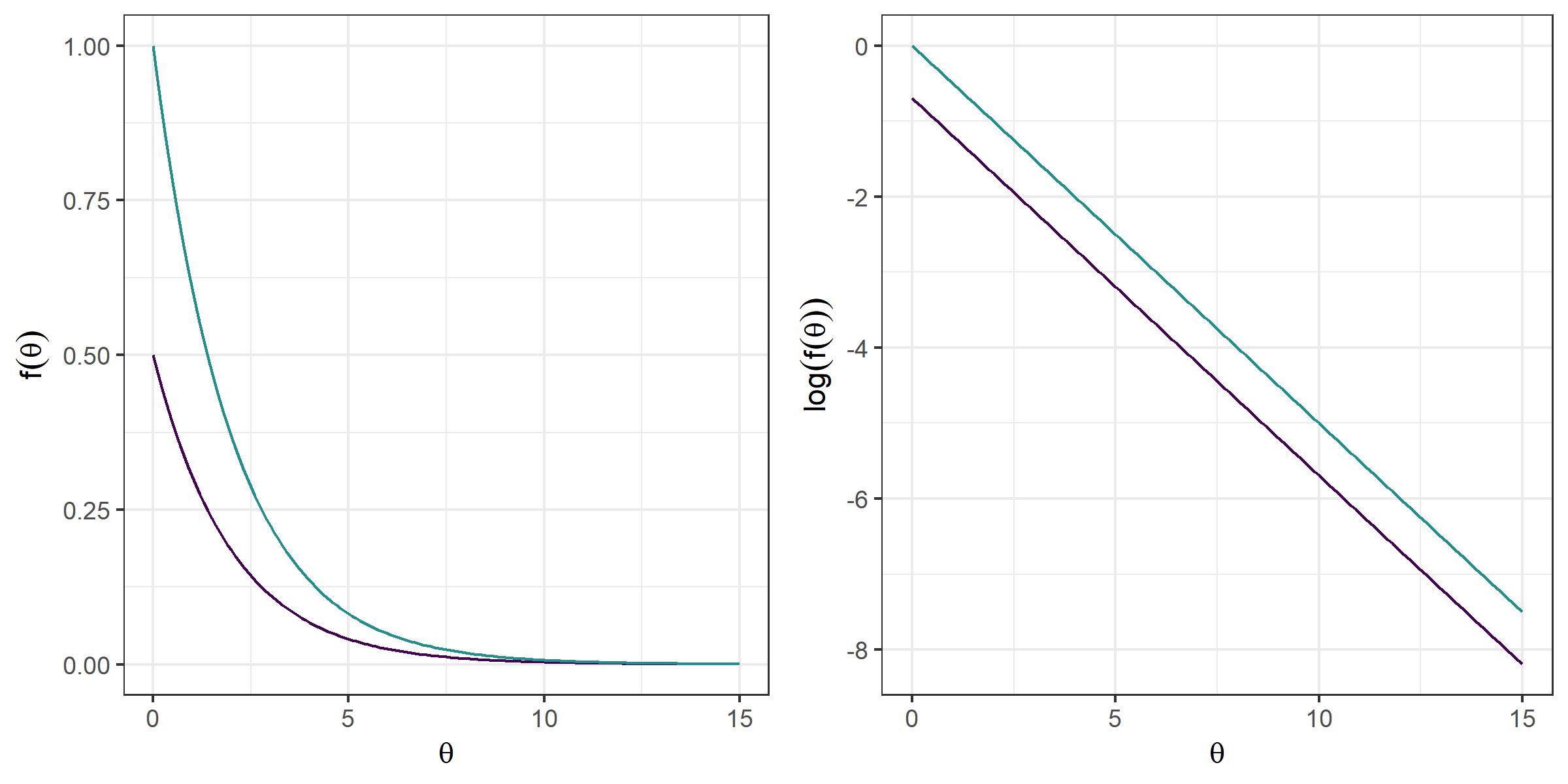
To generate samples, we define the following function:
ar.samps <- function(n) {
   # empty vector to store results

   res <- numeric(n)
   a.rate <- numeric(n)
   # start loop

   for (t in 1:n) {
      # empty NA object

      tmp.res <- NA
      # counter

      iter <- 0
      # loop until u <= r

      while (is.na(tmp.res)) {
         # sample h(theta)

         x <- rexp(1, rate=1/2)
         # sample uniform(0,1)

         u <- runif(1)
         # evaluate

         r <- dchisq(x, 2)/(2 * dexp(x, 1/2))
         # accept if u <= r

         if (u <= r) tmp.res <- x
         # update counter

         iter <- iter + 1
      }
      # if accepted store result

      res[t] <- tmp.res
      a.rate[t] <- 1/iter
   }

   message(paste0('Acceptance rate :',round(mean(a.rate),3)))
   return(res)
}
Now, let’s see whether it works.
# set seed

set.seed(123)
# generate 10000 samples

samps <- ar.samps(10000)
## Acceptance rate :0.699
We might plot the distribution of the samples and compare it to the true density to evaluate whether the method works as expected.
ggplot(data.table(samps),
       aes(x = samps)) +
    geom_histogram(
        bins = 100,
        aes(y = ..density..),
        col = 'white',
        fill = cols[2],
        alpha = .5,
        boundary = 0
    ) +
    geom_line(
        data = data.table(
            x = seq(min(samps), max(samps), .05),
            y = dchisq(seq(min(samps), max(samps), .05), 2)
        ),
        inherit.aes = F,
        aes(x = x, y = y),
        col =  cols[1]
    ) +
    theme_bw() +
    labs(x = expression(theta), y = expression(f(theta)))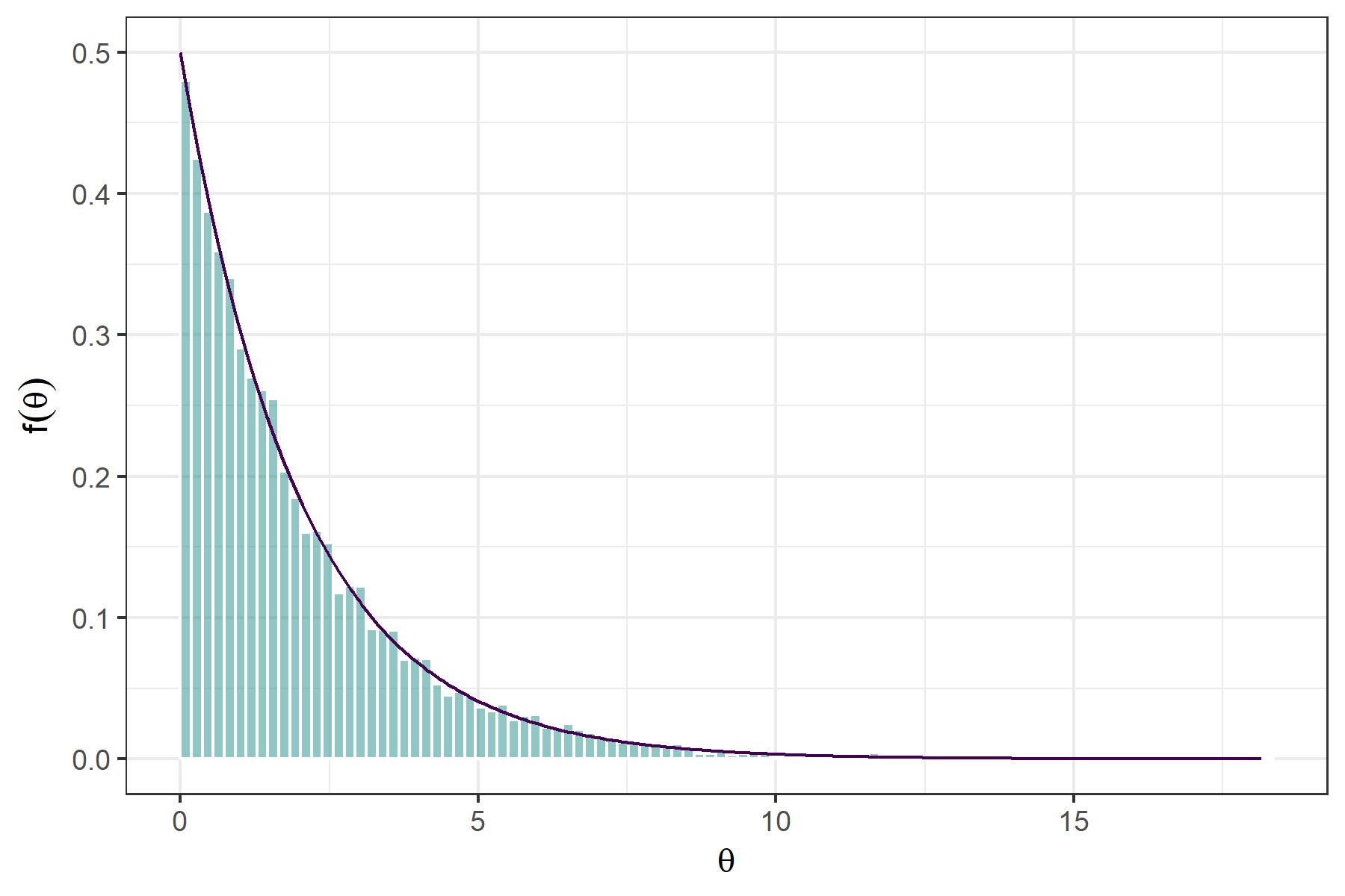
Close! Note that we might improve the acceptance rate by finding a function $ g^* $ which better approximates the chi-squared distribution from above. A great strength of accept-reject sampling is that we will obtain independent samples from the target distribution, which is not the case in MCMC methods.
A clear shortcoming of the Accept-Reject sampling method, on the other hand, is that it is hard to apply in situations where $ \theta $ is multidimensional as it will become increasingly difficult to find a function that will dominate $ p $ for all $ \theta \in \Theta $ which is, in turn, proportional to a distribution from which we can easily sample. Also, there are a lot of situations where a function of the form $ g = k \cdot h $ such that $ \forall \theta \in \Theta, g \ge p $ is difficult to find.